Chapter 13: Control IV – Reinforcement Learning Foundations

13.1 Motivation: From Classical & Optimal Control to Learning-Based Control

In previous chapters, we explored classical and optimal control techniques, such as PID controllers, Linear Quadratic Regulators (LQR), Linear Quadratic Gaussian (LQG) estimators, and Model Predictive Control (MPC). These methods rely on well-defined mathematical models of the system dynamics, often assuming linearity, full state observability, or known disturbances. For instance, PID controllers use proportional, integral, and derivative terms to minimize tracking errors in feedback loops, while LQR optimizes quadratic cost functions for linear systems, and MPC solves constrained optimization problems over a receding horizon. LQG extends LQR to handle noisy measurements via Kalman filtering.

Reinforcement Learning (RL), on the other hand, represents a paradigm shift toward learning-based control. Unlike model-based methods like MPC, which require an explicit system model (e.g., \( \dot{\mathbf{x}} = \mathbf{Ax} + \mathbf{Bu} \)), RL agents learn optimal behaviors through trial-and-error interactions with the environment, guided by rewards. This makes RL particularly advantageous in handling uncertainty, non-linearity, and partial models: common challenges in space engineering.

For example, in orbit control for satellites, classical PID might struggle with unmodeled gravitational perturbations or sensor noise, while LQR/LQG assumes linear dynamics that may not hold for large maneuvers. MPC can address non-linearities, but demands accurate models and significant computational resources for real-time optimization. RL shines here by learning policies that adapt to uncertainties, such as in autonomous station-keeping where the agent can discover fuel-efficient strategies without a perfect dynamics model. Similarly, in space robotics (e.g., manipulator arms on the ISS), RL can handle high-dimensional, non-linear kinematics with partial observability, outperforming traditional methods when models are incomplete or environments are stochastic.

Overall, RL bridges the gap between control theory and machine learning, enabling robust performance in complex, real-world scenarios where traditional approaches may falter due to modeling limitations.

13.1.1 When RL Shines in Engineering

Model-based control techniques (PID, LQR, MPC, etc.) perform extremely well when we possess an accurate, low-to-moderate-dimensional dynamical model and the disturbances are either known or can be adequately captured by simple stochastic descriptions. In many real engineering systems, these assumptions break down in one or more of the following ways:

• Incomplete or highly uncertain dynamics: Atmospheric drag on low-Earth-orbit satellites varies strongly with solar activity and vehicle attitude; flexible appendages introduce unmodeled structural modes; plume impingement in formation flying couples vehicles in ways that are difficult to predict analytically.

• High-dimensional or partially observable state spaces: A planetary rover has dozens of joint angles, wheel slip ratios, and terrain parameters that are never perfectly known. A robotic manipulator on a space station must reason about contact forces, micro-gravity floating base dynamics, and visual occlusions: state dimensions easily exceed hundreds or thousands.

• Complex, long-horizon objectives with sparse rewards: Autonomous docking, debris removal, or in-orbit servicing require sequences of hundreds or thousands of actions where meaningful feedback (success/failure) arrives only at the end of the episode. Classical methods struggle to propagate credit through such long horizons without an excellent predictive model.

• Multi-agent and game-theoretic interactions: Satellite constellations with collision-avoidance negotiations, or cooperative assembly tasks, introduce non-stationary dynamics because each agent’s policy affects the others.

In these regimes, reinforcement learning excels because the agent can discover effective strategies directly from data, even when the true equations of motion are unknown, high-dimensional, or stochastic. Instead of hand-crafting a model and solving an optimization problem online, the RL agent iteratively refines a policy that maps (possibly partial) observations to actions, gradually learning to exploit regularities that were never explicitly modeled.

Some space relevant examples where RL has already shown promise:

• Adaptive station-keeping under uncertain \( J_2 \), drag, and solar-radiation pressure

• Autonomous spacecraft docking and rendezvous with minimal fuel (NASA’s work on RL-based guidance)

• Planetary rover path planning on unknown, slippery regolith

• Dexterous manipulation with soft robotic grippers for on-orbit servicing

13.1.2 Limitations and Practical Considerations

Despite its strengths, reinforcement learning is not a drop-in replacement for classical or optimal control. Engineers adopting RL must be aware of the following fundamental challenges:

Challenge	Description	Space-Specific Implications
Sample inefficiency (in pure from-scratch settings)	While modern variants with demonstrations or priors can learn from few interactions, baseline model-free RL often requires extensive data to explore high-dimensional spaces effectively.	Real spacecraft cannot execute millions of maneuvers; simulation-reality gap (“Sim2Real”) remains critical even with efficient methods.
Exploration risk	Random exploration can drive the system into unsafe or destructive states.	In space, a single bad thrust can de-tumble a satellite or cause collision; physical testing is essentially impossible.
Reward design fragility	Poorly shaped rewards lead to unintended behavior (reward hacking).	Sparse rewards (e.g., “+1 if docked, 0 otherwise”) yield almost no learning signal for long-horizon missions.
Non-stationarity & brittleness	Policies trained in one environment often fail when parameters drift (e.g., mass change after fuel depletion).	Orbital environments evolve (drag coefficient changes, sensor degradation); policies must remain robust or adapt online.
Lack of formal guarantees	Unlike LQR or robust MPC, most RL methods offer no hard stability or constraint-satisfaction certificates.	Certification for flight software is a major barrier in aerospace.

These difficulties explain why pure end-to-end deep RL is still rare on actual flight hardware today. Instead, successful engineering deployments almost always combine RL with prior knowledge: hierarchical architectures, safety shields, model-based initialization, sim2real transfer techniques (domain randomization, system identification), and reward shaping informed by control theory.

While early deep reinforcement learning (RL) methods (e.g., DQN or PPO in high-dimensional tasks like Atari games) often required millions or billions of environment interactions to converge from scratch, recent advances in sample-efficient RL, especially for robotics, have dramatically reduced this requirement. In many cases, particularly when incorporating expert demonstrations, priors, or curricula, RL can learn effective policies from just a few episodes or even a single successful demonstration. For instance, methods like self-imitation RL (SIRL), demonstration-guided exploration, or LLM-augmented RL (e.g., RLingua) enable convergence in under 50 episodes or generations by leveraging structured knowledge or bootstrapping from sparse successes.

The remainder of this chapter (and the next) will equip you with the foundational tools: Markov decision processes, dynamic programming, temporal-difference learning, function approximation, and policy gradients, so that you can understand when and how to responsibly apply RL in computational engineering practice, and where classical methods remain the safer, more efficient choice.

13.2 Markov Decision Processes (MDPs) – The Mathematical Framework

Markov Decision Processes (MDPs) provide the foundational mathematical framework for reinforcement learning (RL), formalizing sequential decision-making under uncertainty. An MDP models an agent’s interaction with an environment as a cycle of observing states, taking actions, receiving rewards, and transitioning to new states. This setup captures the essence of control problems where decisions affect future outcomes, making it ideal for engineering applications like autonomous systems in space.

At its core, an MDP is defined by a tuple \( (S, A, P, R, \gamma) \), where each element represents a key aspect of the decision process. The “Markov” property ensures that the future state depends only on the current state and action, not on prior history: simplifying analysis while still allowing rich dynamics.

A simple space engineering example is satellite attitude control: The satellite must maintain a desired orientation despite disturbances like magnetic torques. Here, the state could include current angles and angular velocities, actions might be thruster firings, transitions account for orbital dynamics, rewards penalize deviation from the target attitude and fuel use, and discounting prioritizes short-term stability.

Below is a conceptual diagram of the MDP interaction loop:

13.2.2 Finite vs. Infinite MDPs

MDPs can be finite (discrete, episodic tasks with termination, like docking maneuvers ending on success/failure) or infinite (continuous spaces, ongoing tasks like perpetual station-keeping).

Finite MDPs suit tabular methods; infinite require approximations (e.g., function approximators for high-dimensional space states). In space applications, hybrid forms are common: episodic for mission phases, continuing for long-duration operations. This framework enables RL to solve underdetermined problems where dynamics are partially known or stochastic.

13.2.1 Components of an MDP

• State Space \( S \): The set of all possible states the environment can be in. States encode relevant information for decision-making. In continuous spaces (common in engineering), \( S \subseteq \mathbb{R}^n \); in discrete, it’s a finite set. For the satellite example, \( s = [\theta, \dot{\theta}]^\top \), where \( \theta \) is attitude error and \( \dot{\theta} \) is rate.

• Action Space \( A \): The set of all possible actions the agent can take. Actions can be discrete (e.g., fire thruster left/right) or continuous (e.g., torque magnitude \( u \in \mathbb{R}^m \)). In attitude control, \( a \) might be a vector of control torques.

• Transition Dynamics \( P(s' | s, a) \): The probability distribution over next states \( s' \) given current state \( s \) and action \( a \). This models the environment’s response, including uncertainty (e.g., stochastic disturbances). In deterministic cases, it’s a function \( s' = f(s, a) \); probabilistically, \( P \) captures noise like sensor errors in space.

• Reward Function \( R(s, a, s') \): A scalar signal indicating the immediate desirability of the transition. Rewards guide learning: positive for good outcomes (e.g., +1 for stable attitude), negative for bad (e.g., -fuel cost or -deviation penalty). In engineering, rewards often encode objectives like minimizing energy while achieving goals.

• Discount Factor \( \gamma \in [0, 1) \): Discounts future rewards to emphasize short-term gains, ensuring convergence in infinite-horizon problems. A \( \gamma \) close to 1 values long-term planning (e.g., fuel-efficient orbits); closer to 0 prioritizes immediacy (e.g., emergency maneuvers). The total return is \( G_t = \sum_{k=0}^\infty \gamma^k r_{t+k+1} \).

13.3 Overview of Reinforcement Learning Methods

For an overview of reinforcement learning (RL) methods from an engineering perspective, we follow the treatment in Chapter 11 of Data-Driven Science and Engineering by Brunton and Kutz provides a comprehensive overview of reinforcement learning (RL) methods, emphasizing their connections to dynamical systems and control theory. A key visual aid is Figure 11.3, which presents a rough categorization of RL algorithms along several dichotomies. This figure helps navigate the diverse landscape of RL techniques by organizing them into overlapping categories based on their underlying principles.

Brunton and Kutz Figure 11.3 provides an overview that classifies RL methods across three primary dimensions:

• Model-based vs. Model-free: One axis distinguishes methods that explicitly build or use a model of the environment’s dynamics from those that learn directly from experience without a model.

• Gradient-based vs. Gradient-free: Another dimension separates algorithms that optimize using gradients (e.g., via backpropagation) from those that do not require derivatives, such as tabular or evolutionary approaches.

• On-policy vs. Off-policy: A third aspect differentiates learning from data generated by the current policy (on-policy) versus data from any policy (off-policy, allowing reuse of old experiences).

Category	Model-Based Examples	Model-Free Examples
Gradient-Based	Model-based policy optimization (e.g., PILCO)	Policy gradients (e.g., REINFORCE, PPO); Actor-Critic (A2C/A3C)
Gradient-Free	Model-based planning (e.g., MCTS with learned models)	Tabular methods (e.g., Q-learning, SARSA); Evolutionary strategies
On-Policy Subset	On-policy model-based (e.g., some MPC variants)	SARSA, REINFORCE
Off-Policy Subset	Off-policy model-based (e.g., Dyna-Q)	Q-learning, DQN

The representative algorithms in each category or intersection are:

• Model-based methods (e.g., Dyna, Model Predictive Control with learned models).

• Model-free methods (e.g., Q-learning, SARSA).

• Gradient-based (e.g., Policy Gradients, Actor-Critic).

• Gradient-free (e.g., Tabular Q-learning, Genetic Algorithms).

• On-policy (e.g., SARSA, REINFORCE).

• Off-policy (e.g., Q-learning, DQN).

Explanations of Key Dichotomies

Below, we briefly define each dichotomy, and elaborate more formally on their meanings and implications for RL algorithm design:

Definition: Model-Based vs. Model-Free: Model-based RL explicitly learns or uses a transition model \( P(s' | s, a) \) and reward function \( R(s, a, s') \) to plan actions (e.g., via simulation or optimization). This connects to optimal control concepts like the Hamilton-Jacobi-Bellman (HJB) equation. Model-free methods, in contrast, learn value functions or policies directly from trial-and-error data without building a model, making them suitable for complex, high-dimensional environments where modeling is intractable.

Definition: Gradient-Based vs. Gradient-Free: Gradient-based methods compute derivatives of a loss or objective (e.g., policy gradient theorem: \( \nabla_\theta J(\theta) = \mathbb{E} [\nabla_\theta \log \pi_\theta(a|s) \hat{A}(s,a)] \)) to update parameters, often using neural networks. Gradient-free approaches avoid derivatives, relying on finite differences, evolutionary algorithms, or tabular lookups—useful when the objective is non-differentiable or black-box.

Definition: On-Policy vs. Off-Policy: -policy learning evaluates and improves the same policy that generates data (e.g., SARSA update: \( Q(s,a) \leftarrow Q(s,a) + \alpha [r + \gamma Q(s',a') - Q(s,a)] \), where \( a' \) comes from the current policy). Off-policy methods learn from data generated by a different (behavior) policy, enabling better data reuse and exploration (e.g., Q-learning: \( Q(s,a) \leftarrow Q(s,a) + \alpha [r + \gamma \max_{a'} Q(s',a') - Q(s,a)] \)).

We will explore the following foundational equations for RL, rooted in the Markov Decision Process (MDP) framework:

• MDP Definition: An MDP (as discussed in 13.2.1) is defined by the tuple \( (S, A, P, R, \gamma) \), where \( S \) is the state space, \( A \) the action space, \( P(s'|s,a) \) the transition probabilities, \( R(s,a,s') \) the reward, and \( \gamma \in [0,1) \) the discount factor.

• Bellman Expectation Equation (for value function under policy \( \pi \)): \( V^\pi(s) = \sum_a \pi(a|s) \left[ R(s,a) + \gamma \sum_{s'} P(s'|s,a) V^\pi(s') \right] \).

• Bellman Optimality Equation (for optimal value \( V^* \)): \( V^*(s) = \max_a \left[ R(s,a) + \gamma \sum_{s'} P(s'|s,a) V^*(s') \right] \).

• Policy Iteration: Alternates evaluation (solve Bellman expectation) and improvement (greedy update: \( \pi(s) = \arg\max_a Q(s,a) \)).

• Value Iteration: Iteratively applies the optimality operator: \( V^{k+1}(s) = \max_a \left[ R(s,a) + \gamma \sum_{s'} P(s'|s,a) V^k(s') \right] \).

• Q-Learning Update (off-policy, model-free): As above, converging to the optimal action-value \( Q^*(s,a) \).

These equations form the mathematical backbone, algorithms like policy/value iteration fit into dynamic programming (model-based, known MDP), while Q-learning extends to unknown environments (model-free).

13.3.1 Model-Based vs. Model-Free RL

In reinforcement learning (RL), a fundamental distinction is between model-based and model-free approaches, which differ in how they handle the environment’s dynamics and learn optimal behaviors. model-based methods are positioned as leveraging explicit models for planning, while model-free methods rely on direct interaction data.

Model-based RL involves learning or using an explicit model of the environment’s dynamics, typically represented as a transition function \( P(s' | s, a) \) (next state given current state and action) and reward function \( R(s, a, s') \). In engineering contexts, this often mirrors classical control formulations, such as the state-space dynamics \( \dot{\mathbf{x}} = f(\mathbf{x}, \mathbf{u}) \), where \( \mathbf{x} \) is the state and \( \mathbf{u} \) the control input. The agent uses this model to simulate trajectories, plan ahead, and optimize policies—similar to model predictive control (MPC). Advantages include higher sample efficiency, as the model allows “mental rehearsals” without real-world interactions. This links directly to optimal control theory, particularly the Hamilton-Jacobi-Bellman (HJB) equation, which solves for the optimal value function \( V^*(\mathbf{x}) = \min_{\mathbf{u}} \left[ c(\mathbf{x}, \mathbf{u}) + \gamma \frac{\partial V^*}{\partial \mathbf{x}} f(\mathbf{x}, \mathbf{u}) \right] \) (continuous-time variant), where \( c \) is the cost. Examples include Dyna (which learns a model from experience and uses it for planning) and Probabilistic Inference for Learning Control (PILCO), which uses Gaussian processes for uncertainty-aware modeling. In space engineering, model-based RL could simulate orbital mechanics under perturbations like \( J_2 \) for efficient station-keeping.

In contrast, model-free RL does not build an explicit dynamics model; instead, it learns value functions (e.g., \( Q(s, a) \)) or policies directly from raw interaction data (states, actions, rewards) through trial-and-error. This data-driven approach is robust to modeling errors and scales to high-dimensional, complex environments where deriving \( f(\mathbf{x}, \mathbf{u}) \) analytically is infeasible. It connects to deep RL, where neural networks approximate functions in methods like Deep Q-Networks (DQN) or Proximal Policy Optimization (PPO), enabling end-to-end learning from pixels (e.g., in robotics vision). However, model-free methods can be sample-inefficient, requiring extensive data to converge. The core mechanism is temporal-difference learning, updating estimates based on bootstrapped values without simulating full trajectories. For instance, Q-learning iteratively refines \( Q(s, a) \) without needing \( P \) or \( R \).

The trade-off is clear: model-based methods excel in structured, low-data regimes with interpretable dynamics (tying to HJB/optimal control for guarantees), but suffer if the model is inaccurate or expensive to learn. Model-free methods shine in unstructured, high-dimensional settings (leveraging deep RL for generalization), but demand more interactions—motivating hybrids like Model-Based Acceleration (MBA) that combine both for space applications, such as adaptive control under uncertain atmospheric drag.

13.3.2 Gradient-Based vs. Gradient-Free Methods

Another key dichotomy in reinforcement learning (RL), is between gradient-based and gradient-free methods. This classification focuses on how algorithms optimize policies or value functions: either by computing explicit gradients for updates or by using derivative-free techniques. Gradient-based approaches are often associated with continuous, differentiable parameterizations (e.g., neural networks), while gradient-free methods are more versatile for discrete or non-differentiable settings.

Gradient-based RL methods optimize a parameterized objective directly using gradients, typically via automatic differentiation and backpropagation. A prime example is policy gradient methods, such as REINFORCE, where the policy \( \pi_\theta(a|s) \) (parameterized by \( \theta \), e.g., neural network weights) is updated to maximize the expected return \( J(\theta) = \mathbb{E}_{\tau \sim \pi_\theta} [R(\tau)] \), with the gradient given by the policy gradient theorem: \( \nabla_\theta J(\theta) = \mathbb{E} [\nabla_\theta \log \pi_\theta(a|s) G_t] \), where \( G_t \) is the return from time \( t \). This enables smooth updates in high-dimensional continuous action spaces, linking to stochastic gradient descent (SGD) in machine learning. Pros include high efficiency in parameter-rich models (e.g., deep networks), as gradients provide directed improvements, leading to faster convergence in smooth landscapes. They are particularly applicable in engineering tasks like continuous control in space systems, such as optimizing thrust vectors for satellite attitude adjustment, where policies can be fine-tuned for precision. However, cons involve sensitivity to non-differentiable elements (e.g., discrete actions or hard constraints) and potential instability from noisy gradients in sparse-reward environments.

In contrast, gradient-free RL methods avoid computing derivatives altogether, relying on sampling, perturbations, or tabular updates to explore and evaluate options. Classic examples include Q-learning (a gradient-free value-based method), which updates the action-value function \( Q(s,a) \) via temporal differences without gradients: \( Q(s,a) \leftarrow Q(s,a) + \alpha [r + \gamma \max_{a'} Q(s',a') - Q(s,a)] \), or evolutionary strategies that treat policies as black-box functions and evolve populations via mutations. These are often tabular or use finite differences for approximation. Pros emphasize broad applicability: they handle non-differentiable, discrete, or black-box objectives seamlessly, making them robust in uncertain or hybrid systems (e.g., spacecraft with switched modes like thruster on/off). They also avoid local optima traps common in gradient descent by leveraging global exploration. Cons center on lower efficiency, especially in high-dimensional spaces, as they require many evaluations (e.g., rollouts) without directional guidance, leading to higher sample complexity: critical in space engineering where simulations are computationally expensive.

Overall, gradient-based methods (e.g., policy gradients like PPO or TRPO) excel in efficiency for scalable, continuous problems with deep RL integration, but demand differentiability. Gradient-free approaches (e.g., Q-learning or cross-entropy methods) prioritize flexibility and robustness, suiting discrete or model-agnostic scenarios, though at the cost of data hunger. Hybrids, such as gradient-free wrappers around gradient-based cores, offer compromises for real-world applications like autonomous rover navigation under variable terrain.

13.3.3 On-Policy vs. Off-Policy Learning

A third important dichotomy in reinforcement learning (RL) is between on-policy and off-policy methods. This classification centers on the relationship between the policy used to generate data (for exploration and interaction) and the policy being learned or improved. On-policy approaches tie learning directly to the current policy’s behavior, while off-policy methods decouple data generation from policy optimization, enabling more flexible use of experiences. This distinction has significant implications for exploration strategies and data efficiency, particularly in engineering applications where real-world interactions are costly or risky.

On-policy RL methods learn and evaluate the value function or policy using data generated exclusively by the current policy being optimized. In other words, the agent acts according to its present policy \( \pi \), collects trajectories (states, actions, rewards), and updates \( \pi \) based on those same trajectories. This creates a self-consistent loop where improvements are grounded in the policy’s own behavior. Key examples include:

• SARSA (State-Action-Reward-State-Action): An on-policy temporal-difference (TD) method for action-value learning. The update rule is \( Q(s,a) \leftarrow Q(s,a) + \alpha [r + \gamma Q(s',a') - Q(s,a)] \), where \( a' \) is sampled from the current policy \( \pi \) (e.g., ε-greedy). This ensures the update reflects the policy’s exploratory actions.

• TD(0): A basic on-policy algorithm for state-value estimation, updating \( V(s) \leftarrow V(s) + \alpha [r + \gamma V(s') - V(s)] \) based on samples from \( \pi \).

On-policy methods promote consistent learning but require the policy itself to handle exploration (e.g., via softmax or ε-greedy), which can lead to suboptimal data if exploration is too aggressive or conservative. Data usage is limited to fresh trajectories from the current \( \pi \), making these methods less sample-efficient but easier to implement with guarantees of convergence under certain conditions.

In contrast, off-policy RL methods learn a target policy \( \pi \) from data generated by a different behavior policy \( \mu \) (where \( \mu \neq \pi \)). This separation allows the agent to explore broadly with \( \mu \) (e.g., a random or exploratory policy) while optimizing \( \pi \) toward optimality (e.g., greedy). Corrections like importance sampling ratios \( \frac{\pi(a|s)}{\mu(a|s)} \) adjust for the policy mismatch. Prominent examples are:

• Q-learning: A foundational off-policy TD method, with the update \( Q(s,a) \leftarrow Q(s,a) + \alpha [r + \gamma \max_{a'} Q(s',a') - Q(s,a)] \). Here, the max assumes a greedy target policy, even if the behavior policy is exploratory.

• Deep Q-Networks (DQN): An off-policy deep RL extension of Q-learning, using neural networks for \( Q \)-approximation, experience replay buffers to store and reuse diverse data, and target networks for stability.

Off-policy approaches enhance exploration by allowing \( \mu \) to be designed independently for safety or coverage (e.g., more random in simulations), while \( \pi \) focuses on exploitation. For data usage, they excel in efficiency by replaying historical experiences from any policy, reducing the need for constant new interactions which is critical in high-cost domains like space engineering.

Implications for Exploration and Data Usage:

• Exploration: On-policy methods integrate exploration into the policy, which can bias learning toward safer but suboptimal paths (e.g., SARSA learns a “cautious” policy avoiding cliffs in gridworlds). Off-policy methods (e.g., Q-learning) enable aggressive exploration via \( \mu \) without corrupting \( \pi \), ideal for space scenarios like satellite maneuvering where real trials risk collisions but simulations can explore freely.

• Data Usage: On-policy requires discarding old data when \( \pi \) changes, leading to waste in dynamic environments. Off-policy leverages replay buffers for better sample efficiency, though it introduces variance from importance sampling. In practice, off-policy is preferred for data-scarce engineering tasks (e.g., rover path planning with limited battery life), but on-policy offers simplicity and stability in well-modeled systems.

This flexibility makes off-policy methods like DQN prevalent in deep RL for complex, partially observable space applications, while on-policy variants suit iterative refinement in known dynamics. Hybrids, such as importance-sampled actor-critic, often balance these trade-offs in real-world deployments.

13.4 Policies, Value Functions, and Bellman Equations

In reinforcement learning (RL), the agent’s decision-making strategy is captured by a policy, while value functions quantify the long-term desirability of states or state-action pairs under that policy. These concepts build on the MDP framework, enabling the agent to evaluate and improve behaviors to maximize cumulative rewards. Policies map states to actions, and value functions provide a scalar measure of expected future rewards, forming the basis for learning algorithms.

A policy \( \pi(a|s) \) specifies the probability of taking action \( a \) in state \( s \). The state-value function \( V^\pi(s) \) estimates the expected return starting from state \( s \) and following policy \( \pi \): \( V^\pi(s) = \mathbb{E}_\pi \left[ \sum_{k=0}^\infty \gamma^k r_{t+k+1} \bigg| s_t = s \right], \) where the expectation is over trajectories generated by \( \pi \), and \( \gamma \) is the discount factor.

The action-value function \( Q^\pi(s,a) \) similarly estimates the expected return starting from \( s \), taking action \( a \), and then following \( \pi \): \( Q^\pi(s,a) = \mathbb{E}_\pi \left[ \sum_{k=0}^\infty \gamma^k r_{t+k+1} \bigg| s_t = s, a_t = a \right]. \) These relate via \( V^\pi(s) = \sum_a \pi(a|s) Q^\pi(s,a) \).

The Bellman expectation equation expresses value functions recursively, leveraging the MDP’s Markov property:

For \( V^\pi \): \( V^\pi(s) = \sum_a \pi(a|s) \sum_{s', r} P(s',r | s,a) \left[ r + \gamma V^\pi(s') \right], \) where the inner sum is over possible next states and rewards (often simplified if rewards are deterministic).

For \( Q^\pi \): \( Q^\pi(s,a) = \sum_{s', r} P(s',r | s,a) \left[ r + \gamma \sum_{a'} \pi(a'|s') Q^\pi(s',a') \right]. \)

The Bellman optimality equation defines optimal values \( V^*(s) = \max_\pi V^\pi(s) \) and \( Q^*(s,a) = \max_\pi Q^\pi(s,a) \):

\( V^*(s) = \max_a \sum_{s', r} P(s',r | s,a) \left[ r + \gamma V^*(s') \right], \) \( Q^*(s,a) = \sum_{s', r} P(s',r | s,a) \left[ r + \gamma \max_{a'} Q^*(s',a') \right]. \)

These equations are derived by noting that optimal policies choose actions greedily with respect to the optimal values, forming a system of nonlinear equations solvable via iterative methods (as in dynamic programming). In engineering contexts, like spacecraft control, these enable computing optimal thrust policies under fuel constraints.

13.4.1 Policy Types and Evaluation

Policies come in two main types: deterministic and stochastic. A deterministic policy \( \pi(s) \) maps each state \( s \) to a single action \( a \), i.e., \( \pi(a|s) = 1 \) for one \( a \) and 0 otherwise—useful in predictable environments like precise orbital maneuvers where exploration is minimal. A stochastic policy \( \pi(a|s) \) assigns probabilities to actions, enabling inherent exploration (e.g., via softmax over Q-values), which is crucial in uncertain settings like rover navigation on variable terrain to avoid local optima. Policy evaluation computes \( V^\pi \) or \( Q^\pi \) for a fixed policy, often using the Bellman expectation equation iteratively. Starting with an initial guess (e.g., \( V_0(s) = 0 \)), updates are: \( V_{k+1}(s) = \sum_a \pi(a|s) \sum_{s', r} P(s',r | s,a) \left[ r + \gamma V_k(s') \right]. \) This converges to \( V^\pi \) as \( k \to \infty \) for finite MDPs (by contraction mapping). In practice, it’s used in policy iteration or as a subroutine in actor-critic methods, evaluating how well a policy performs in tasks like attitude stabilization.

13.4.2 Optimal Policies and Values

An optimal policy \( \pi^* \) achieves the highest possible values: \( V^{\pi^*}(s) = V^*(s) \) for all \( s \). Multiple optimal policies may exist, but all share the same optimal values. The Bellman optimality equation provides a way to solve for \( V^* \) and \( Q^* \) without enumerating policies, by treating it as a fixed-point problem. Solving involves methods like value iteration: Initialize \( V_0(s) = 0 \), then:

\( V_{k+1}(s) = \max_a \sum_{s', r} P(s',r | s,a) \left[ r + \gamma V_k(s') \right], \)

converging to \( V^* \). Once \( V^* \) (or \( Q^* \)) is known, an optimal policy is extracted greedily: \( \pi^*(s) = \arg\max_a Q^*(s,a) \). For Q-values, the update is analogous. In space engineering, this yields fuel-optimal trajectories (e.g., for rendezvous), but requires a known MDP model. In unknown environments, approximations extend this to model-free RL, balancing computation with performance.

13.5 Dynamic Programming – Solving Known MDPs

Dynamic Programming (DP) methods provide exact solutions for MDPs where the model (transitions \( P \) and rewards \( R \)) is fully known. These algorithms break down the Bellman equations into iterative procedures to compute optimal values and policies, serving as a foundation for more advanced RL in unknown environments. In engineering, DP is useful for offline planning in simulated systems, like optimizing spacecraft trajectories with known orbital dynamics.

Policy Evaluation

Policy evaluation computes the value function \( V^\pi \) for a fixed policy \( \pi \), solving the linear system from the Bellman expectation equation: \( V^\pi(s) = \sum_a \pi(a|s) \sum_{s'} P(s'|s,a) \left[ R(s,a,s') + \gamma V^\pi(s') \right]. \) Iteratively, start with \( V_0(s) = 0 \) and update: \( V_{k+1}(s) = \sum_a \pi(a|s) \sum_{s'} P(s'|s,a) \left[ R(s,a,s') + \gamma V_k(s') \right], \) until convergence (e.g., \( \|V_{k+1} - V_k\| < \epsilon \)). This evaluates policy performance, e.g., assessing fuel efficiency in a given satellite control strategy.

Policy Improvement

Given \( V^\pi \), improve the policy greedily: For each \( s \), set \( \pi'(s) = \arg\max_a Q^\pi(s,a) \), where \( Q^\pi(s,a) = \sum_{s'} P(s'|s,a) \left[ R(s,a,s') + \gamma V^\pi(s') \right]. \) This yields a better or equal policy \( \pi' \geq \pi \), as per the policy improvement theorem: crucial for refining suboptimal initial policies in control tasks.

Policy Iteration

Policy iteration alternates evaluation and improvement until the policy stabilizes:

1. Initialize arbitrary policy \( \pi_0 \).

2. Evaluate: Compute \( V^{\pi_k} \).

3. Improve: Set \( \pi_{k+1}(s) = \arg\max_a Q^{\pi_k}(s,a) \).

4. Repeat until \( \pi_{k+1} = \pi_k \). This converges to \( \pi^* \) in finite steps for finite MDPs, balancing computation in applications like optimal path planning for rovers.

Value Iteration

Value iteration directly solves the Bellman optimality equation iteratively: \( V_{k+1}(s) = \max_a \sum_{s'} P(s'|s,a) \left[ R(s,a,s') + \gamma V_k(s') \right], \) converging to \( V^* \). Extract \( \pi^* \) greedily from \( V^* \). It’s simpler (no full evaluations) but may require more iterations; efficient for large state spaces in simulated space missions.

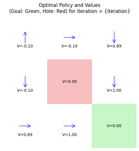
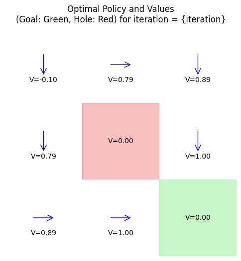
Example: Small Gridworld Example

Consider a 3x3 gridworld (states 0-8, row-major): Start at 0, goal at 8 (+1 reward), hole at 4 (-1 reward, terminal).

Actions: up, down, left, right (deterministic, but clip at edges). \( \gamma = 0.9 \).

DP finds a policy avoiding the hole while reaching the goal efficiently, analogous to rover navigation avoiding craters.

Below is a Python implementation of tabular policy iteration on this MDP, enhanced with a visualization function using Matplotlib to display the grid, policy arrows, and value labels. (For value iteration, modify the loop to use the max operator directly.) When run in a Jupyter notebook, this will produce a plot showing the optimal policy and values overlaid on the grid.

import numpy as np
import matplotlib.pyplot as plt
from matplotlib.patches import FancyArrowPatch, Rectangle

# Define MDP: 3x3 grid, states 0-8
num_states = 9
num_actions = 4  # 0: up, 1: down, 2: left, 3: right
gamma = 0.9
theta = 1e-4  # convergence threshold

# Transitions: next_state[s, a], assume deterministic
next_state = np.array([
    # up, down, left, right for each state
    [0, 3, 0, 1],  # s0
    [1, 4, 0, 2],  # s1
    [2, 5, 1, 2],  # s2
    [0, 6, 3, 4],  # s3
    [4, 7, 3, 5],  # s4 (hole)
    [2, 8, 4, 5],  # s5
    [3, 6, 6, 7],  # s6
    [4, 7, 6, 8],  # s7
    [5, 8, 7, 8]   # s8 (goal)
])

# Rewards: r[s, a] = -0.01 step cost, +1 goal, -1 hole
rewards = -0.01 * np.ones((num_states, num_actions))
# Goal transitions to 8 give +1, to 4 give -1
for s in range(num_states):
    for a in range(num_actions):
        if next_state[s, a] == 8:
            rewards[s, a] = 1.0
        elif next_state[s, a] == 4:
            rewards[s, a] = -1.0

# Terminals
terminals = [4, 8]

def policy_evaluation(policy, V):
    while True:
        delta = 0
        for s in range(num_states):
            if s in terminals:
                continue
            v = V[s]
            a = policy[s]
            s_next = next_state[s, a]
            r = rewards[s, a]
            V[s] = r + gamma * V[s_next]
            delta = max(delta, abs(v - V[s]))
        if delta < theta:
            break
    return V

def policy_improvement(policy, V):
    policy_stable = True
    for s in range(num_states):
        if s in terminals:
            continue
        old_a = policy[s]
        Q = np.zeros(num_actions)
        for a in range(num_actions):
            s_next = next_state[s, a]
            r = rewards[s, a]
            Q[a] = r + gamma * V[s_next]
        policy[s] = np.argmax(Q)
        if old_a != policy[s]:
            policy_stable = False
    return policy, policy_stable

# Visualization function
def visualize_grid(policy, V, iteration=0):
    fig, ax = plt.subplots(figsize=(6, 6))
    ax.set_xlim(0, 3)
    ax.set_ylim(0, 3)
    ax.set_xticks(np.arange(4))
    ax.set_yticks(np.arange(4))
    ax.grid(True)

    # Arrow directions: up, down, left, right
    arrows = [(0, 0.3), (0, -0.3), (-0.3, 0), (0.3, 0)]
    labels = ['↑', '↓', '←', '→']

    for i in range(3):
        for j in range(3):
            s = i * 3 + j
            x, y = j + 0.5, 2.5 - i  # Center of cell (row-major, flip y for top-left start)

            # Background colors: goal green, hole red, others white
            color = 'white'
            if s == 8:
                color = 'lightgreen'
            elif s == 4:
                color = 'lightcoral'
            ax.add_patch(Rectangle((j, 2-i), 1, 1, color=color, alpha=0.5))

            if s in terminals:
                ax.text(x, y, f'V={V[s]:.2f}', ha='center', va='center', fontsize=10)
                continue

            # Policy arrow or label
            a = policy[s]
            if arrows[a] != (0,0):  # Draw arrow if applicable
                dx, dy = arrows[a]
                ax.add_patch(FancyArrowPatch((x - dx/2, y - dy/2), (x + dx/2, y + dy/2),
                                             arrowstyle='->', mutation_scale=20, color='blue'))
            else:
                ax.text(x, y + 0.2, labels[a], ha='center', va='center', fontsize=20)

            # Value label
            ax.text(x, y - 0.2, f'V={V[s]:.2f}', ha='center', va='center', fontsize=10)

    ax.set_title('Optimal Policy and Values\n(Goal: Green, Hole: Red) for iteration = {iteration}')
    plt.axis('off')
    plt.show()

# Initialize
policy = np.zeros(num_states, dtype=int)  # arbitrary initial policy
V = np.zeros(num_states)

# Policy Iteration
iteration = 0
while True:
    # Visaulize current policy and values:
    visualize_grid(policy, V, iteration=iteration)
    # Policy Evaluation and Improvement
    V = policy_evaluation(policy, V)
    policy, stable = policy_improvement(policy, V)
    print(f'iteration {iteration}: policy = {policy}, V = {V}')
    iteration += 1
    if stable:
        break
    # Visualize


# Print results
print("Optimal Policy (0=up,1=down,2=left,3=right):", policy)
print("Optimal Values:", V)

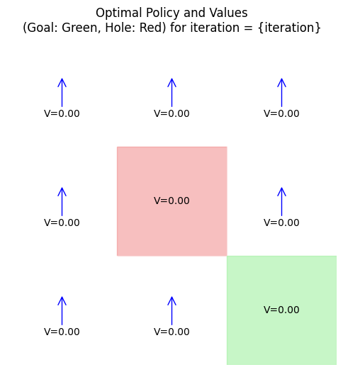
iteration 0: policy = [0 0 0 0 0 1 0 3 0], V = [-0.0991272  -0.0991272  -0.0991272  -0.09921448  0.         -0.09921448
 -0.09929303 -1.          0.        ]

iteration 1: policy = [0 0 1 0 0 1 3 3 0], V = [-0.09929303 -0.09929303 -0.09929303 -0.09936373  0.          1.
 -0.09942736  1.          0.        ]

iteration 2: policy = [0 3 1 1 0 1 3 3 0], V = [-0.09942736 -0.09942736  0.89       -0.09948462  0.          1.
  0.89        1.          0.        ]

iteration 3: policy = [1 3 1 1 0 1 3 3 0], V = [-0.09953616  0.791       0.89        0.791       0.          1.
  0.89        1.          0.        ]

iteration 4: policy = [1 3 1 1 0 1 3 3 0], V = [0.7019 0.791  0.89   0.791  0.     1.     0.89   1.     0.    ]
Optimal Policy (0=up,1=down,2=left,3=right): [1 3 1 1 0 1 3 3 0]
Optimal Values: [0.7019 0.791  0.89   0.791  0.     1.     0.89   1.     0.    ]

13.5.1 Policy Evaluation and Improvement

Policy evaluation and improvement are the core building blocks of dynamic programming in MDPs, enabling systematic computation of values and refinement of policies.

Iterative backups form the basis of policy evaluation. These are recursive updates that “back up” value estimates from future states to the current one, exploiting the Bellman expectation equation. Starting from an arbitrary initial value function (often zero), each iteration sweeps through all states, updating \( V(s) \) based on the expected reward and discounted future value under the current policy. This process is a contraction mapping in the space of value functions, guaranteeing convergence to the true \( V^\pi \) in finite MDPs due to the discount factor \( \gamma < 1 \). In engineering terms, backups propagate long-term consequences (e.g., cumulative fuel costs in orbit control) backward, providing a holistic assessment.

Greedy improvement then refines the policy by selecting actions that maximize the one-step lookahead value. Given \( V^\pi \), compute the action-value \( Q^\pi(s,a) \) for each action, and update the policy to \( \pi'(s) = \arg\max_a Q^\pi(s,a) \). The policy improvement theorem ensures \( V^{\pi'} \geq V^\pi \) (with equality only if \( \pi \) is already optimal), driving monotonic progress. This greediness assumes a known model, making it efficient for deterministic systems like robotic path planning, but it can get stuck in local optima if not iterated.

Together, these steps enable bootstrapping: evaluation uses self-consistent backups, while improvement exploits them for better decisions, forming the foundation for full algorithms.

13.5.2 Policy Iteration Algorithm

The policy iteration algorithm combines evaluation and improvement in a loop to find the optimal policy \( \pi^* \).

Full Algorithm Steps:

1. Initialization: Start with an arbitrary policy \( \pi_0 \) (e.g., random actions) and optional initial values \( V_0(s) = 0 \).

2. Policy Evaluation: Compute \( V^{\pi_k} \) by iteratively solving the Bellman expectation until convergence (or for a fixed number of sweeps in approximate versions).

3. Policy Improvement: For each state, set \( \pi_{k+1}(s) = \arg\max_a \sum_{s'} P(s'|s,a) [R(s,a,s') + \gamma V^{\pi_k}(s')] \).

4. Convergence Check: If \( \pi_{k+1} = \pi_k \) (no changes), stop; else, set \( k \leftarrow k+1 \) and repeat from step 2.

Convergence: In finite MDPs, policy iteration converges to \( \pi^* \) in a finite number of iterations (often few, as each improvement is significant). The number is at most \( |A|^{|S|} \), but practically much less due to monotonicity. This makes it suitable for small-to-medium MDPs in engineering, like discrete approximations of control problems (e.g., quantized satellite states).

In the gridworld example from Section 13.5, the code already implements policy iteration. Here’s a snippet highlighting the loop:

# Policy Iteration Loop
while True:
    V = policy_evaluation(policy, V)  # Step 2: Evaluate
    policy, stable = policy_improvement(policy, V)  # Step 3: Improve
    if stable:  # Step 4: Check
        break

This iterates until stability, yielding the optimal policy and values.

13.5.3 Value Iteration as a Special Case

Value iteration is a streamlined variant of policy iteration, merging evaluation and improvement into a single update rule for faster implementation in some cases.

Differences: Unlike policy iteration’s full evaluation (multiple sweeps until convergence per policy), value iteration performs only one backup per iteration, directly applying the Bellman optimality operator:

\( V_{k+1}(s) = \max_a \sum_{s'} P(s'|s,a) [R(s,a,s') + \gamma V_k(s')]. \) No explicit policy is maintained during iteration; instead, it’s extracted at the end via \( \pi^*(s) = \arg\max_a Q^*(s,a) \) from the converged \( V^* \). This avoids intermediate policies but may require more total iterations since updates are partial. Policy iteration is “policy-centric” with potentially fewer outer loops; value iteration is “value-centric” and simpler to code.

When to Use: Choose value iteration for large state spaces where full evaluations are costly (e.g., discretized PDEs in continuum control), or when early stopping with approximate values suffices. Policy iteration shines when evaluations are cheap and quick convergence in policy space is needed (e.g., small MDPs like attitude control modes). Both are exact in the limit, but value iteration’s asynchronous variants (prioritized sweeping) adapt well to sparse transitions in space applications. To extend the Python example from Section 13.5 to value iteration, replace the main loop with:

# Value Iteration
V = np.zeros(num_states)
while True:
    delta = 0
    for s in range(num_states):
        if s in terminals:
            continue
        v = V[s]
        Q = np.zeros(num_actions)
        for a in range(num_actions):
            s_next = next_state[s, a]
            r = rewards[s, a]
            Q[a] = r + gamma * V[s_next]
        V[s] = np.max(Q)
        delta = max(delta, abs(v - V[s]))
    if delta < theta:
        break


# Extract policy
policy = np.zeros(num_states, dtype=int)
for s in range(num_states):
    if s in terminals:
        continue
    Q = np.zeros(num_actions)
    for a in range(num_actions):
        s_next = next_state[s, a]
        r = rewards[s, a]
        Q[a] = r + gamma * V[s_next]
    policy[s] = np.argmax(Q)



# Reuse visualization
visualize_grid(policy, V)

This converges to the same optima, demonstrating the equivalence.

13.6 Model-Free Methods: Monte-Carlo and Temporal-Difference Learning

Model-free reinforcement learning methods learn optimal policies and values directly from interaction data without building an explicit model of the environment’s dynamics. Two key approaches are Monte-Carlo (MC) methods, which average returns over complete episodes, and Temporal-Difference (TD) learning, which updates estimates incrementally using bootstrapping. MC requires waiting for episode termination to compute full returns, making it unbiased but high-variance, while TD learns from incomplete sequences, reducing variance at the cost of some bias. These are advantageous in unknown or complex environments, such as space systems with unmodeled perturbations (e.g., variable solar radiation on satellites), where deriving transitions analytically is impractical. Model-free methods enable adaptive control, like real-time adjustment in rover navigation or attitude stabilization under uncertainty.

13.6.1 Monte-Carlo Policy Evaluation and Control

Monte-Carlo (MC) methods estimate values by averaging observed returns over many episodes, treating each as a sample from the policy’s distribution. For policy evaluation, the state-value \( V(s) \) is updated as the mean return following first visits (or every visit) to \( s \). First-visit MC averages only the return from the initial occurrence of \( s \) per episode to ensure unbiased estimates; every-visit includes all occurrences, potentially faster converging but biased in overlapping trajectories. For control (optimizing the policy), MC extends to action-values \( Q(s,a) \), but requires exploration to visit all state-action pairs. Techniques include exploring starts (randomly initializing episodes across states/actions, feasible in simulations) or ε-greedy policies (choosing the best action with probability 1-ε, random otherwise, with ε decaying over time). In space engineering, MC control suits episodic tasks like docking maneuvers, where full simulation rollouts estimate fuel-efficient strategies. Below is a Python example of every-visit MC control with ε-greedy exploration on Gymnasium’s Blackjack environment (states: player’s sum, dealer’s card, usable ace; actions: hit/stick; goal: beat dealer without busting).

import gymnasium as gym
import numpy as np
import matplotlib.pyplot as plt

# Initialize environment
env = gym.make('Blackjack-v1')

# Parameters
num_episodes = 100000
epsilon = 0.1  # exploration probability
gamma = 1.0    # no discount (episodic)

# Q-table: states (player_sum 12-21, dealer_card 1-10, usable_ace 0/1) -> actions (0:stick, 1:hit)
# Gym Blackjack states: (player_sum, dealer_showing, usable_ace)
state_space = (10, 10, 2)  # player 12-21 (index 0-9), dealer 1-10 (0-9), ace 0/1
Q = np.zeros(state_space + (2,))
counts = np.zeros(state_space + (2,))  # for averaging

def state_to_index(state):
    player_sum, dealer_card, usable_ace = state
    return (player_sum - 12, dealer_card - 1, int(usable_ace))

def epsilon_greedy_policy(state, epsilon):
    if np.random.rand() < epsilon:
        return np.random.randint(2)  # random action
    idx = state_to_index(state)
    return np.argmax(Q[idx])

# Track episode returns
episode_returns = []  # New list for per-episode returns
avg_returns = []      # For plotting averages every 100 episodes

# MC Control
for episode in range(num_episodes):
    trajectory = []  # (state, action, reward)
    state, _ = env.reset()
    done = False
    while not done:
        action = epsilon_greedy_policy(state, epsilon)
        next_state, reward, done, _, _ = env.step(action)
        trajectory.append((state, action, reward))
        state = next_state

    # Compute episode return (sum of rewards; in Blackjack, equals final reward)
    ep_return = sum(r for _, _, r in trajectory)
    episode_returns.append(ep_return)

    # Compute returns backward for updates
    G = 0
    for t in reversed(range(len(trajectory))):
        state, action, reward = trajectory[t]
        G = reward + gamma * G
        idx = state_to_index(state)
        counts[idx + (action,)] += 1
        Q[idx + (action,)] += (G - Q[idx + (action,)]) / counts[idx + (action,)]

    # Track average return every 100 episodes
    if episode % 100 == 0:
        if episode >= 100:
            avg_returns.append(np.mean(episode_returns[-100:]))
        else:
            avg_returns.append(0)  # Placeholder for early episodes

# Plot learning curve
plt.plot(avg_returns)
plt.xlabel('Episodes (x100)')
plt.ylabel('Average Return (last 100 episodes)')
plt.title('MC Control on Blackjack')
plt.show()

# Optimal policy example (for visualization, e.g., no ace)
policy_no_ace = np.argmax(Q[:, :, 0], axis=2)  # 0: stick, 1: hit
print("Policy (no ace):", policy_no_ace)

---------------------------------------------------------------------------
ModuleNotFoundError                       Traceback (most recent call last)
Cell In[3], line 1
----> 1 import gymnasium as gym
      2 import numpy as np
      3 import matplotlib.pyplot as plt

ModuleNotFoundError: No module named 'gymnasium'

This code learns a near-optimal policy (e.g., hit below ~17, stick above), with the plot showing improving returns.

13.6.2 Temporal-Difference Learning Basics

Temporal-Difference (TD) learning updates value estimates incrementally after each step, without waiting for episode ends. The core idea is bootstrapping: using current estimates to update others, blending MC’s empirical averaging with DP’s recursion.

TD(0) evaluation for \( V^\pi(s) \) uses the update:

\[ V(s) \leftarrow V(s) + \alpha [r + \gamma V(s') - V(s)], \]

where \( r + \gamma V(s') \) is the TD target, and \( \alpha \) is the learning rate. This reduces variance compared to MC (by bootstrapping) but introduces bias (from imperfect estimates). Convergence requires decreasing \( \alpha \) and sufficient exploration under the policy.

A brief mention of eligibility traces: In TD(λ), traces credit recent states/actions with decaying eligibility \( e(s) = \gamma \lambda e(s) + 1 \), extending updates backward for faster propagation in long-horizon tasks like orbit control. TD shines in continuing space environments, enabling online learning amid ongoing disturbances.

13.6.3 On-Policy TD Control: SARSA

SARSA (State-Action-Reward-State-Action) is an on-policy TD control method that learns the action-value function \( Q^\pi(s,a) \) directly. It generates data using the current policy (e.g., ε-greedy) and updates based on the next action from that policy, making it suitable for learning safe, exploratory behaviors.

Algorithm:

• Step 1: Initialize \( Q(s,a) = 0 \) for all \( s,a \).

• Step 2: For each episode:

• \(~\) Start with state \( s \), choose \( a \) from policy (e.g., ε-greedy on \( Q \)).

• \(~\) While not terminal:

• \(~\) \(~\) Take \( a \), observe \( r, s' \).

• \(~\) \(~\) Choose next action \( a' \) from policy.

• \(~\) \(~\) Update: \( Q(s,a) \leftarrow Q(s,a) + \alpha [r + \gamma Q(s',a') - Q(s,a)] \).

• \(~\) \(~\) Set \( s \leftarrow s' \), \( a \leftarrow a' \).

• Step 3: Decay ε over time for greedier policy.

The update rule reflects the policy’s behavior, leading to “cautious” optima (e.g., avoiding risky shortcuts). In space, SARSA suits on-policy adaptation, like thruster control under noise.

Example: SARSA on CliffWalking Environment

Below is a Python example of tabular SARSA on Gymnasium’s CliffWalking environment (4x12 grid; start at (3,0), goal (3,11); cliff at (3,1-10) gives -100 and reset; actions: up/down/left/right).

import gymnasium as gym
import numpy as np
import matplotlib.pyplot as plt
from matplotlib.patches import FancyArrowPatch, Rectangle

env = gym.make('CliffWalking-v1')
num_episodes = 500
alpha = 0.5
gamma = 1.0
epsilon = 0.1

# Q-table: 48 states (4x12 grid), 4 actions (0:up, 1:right, 2:down, 3:left)
Q = np.zeros((env.observation_space.n, env.action_space.n))

episode_rewards = []
for episode in range(num_episodes):
    state, _ = env.reset()
    action = np.argmax(Q[state]) if np.random.rand() > epsilon else env.action_space.sample()
    total_reward = 0
    done = False
    while not done:
        next_state, reward, done, _, _ = env.step(action)
        next_action = np.argmax(Q[next_state]) if np.random.rand() > epsilon else env.action_space.sample()
        Q[state, action] += alpha * (reward + gamma * Q[next_state, next_action] - Q[state, action])
        state, action = next_state, next_action
        total_reward += reward
    episode_rewards.append(total_reward)

# Plot rewards
plt.figure(figsize=(8, 4))
plt.plot(episode_rewards)
plt.xlabel('Episode')
plt.ylabel('Total Reward')
plt.title('SARSA Learning Curve on CliffWalking')
plt.show()

# Extract policy and values (max Q per state)
policy = np.argmax(Q, axis=1)
values = np.max(Q, axis=1)

# Visualization function
def visualize_cliff_policy(policy, values):
    rows, cols = 4, 12
    fig, ax = plt.subplots(figsize=(12, 4))
    ax.set_xlim(0, cols)
    ax.set_ylim(0, rows)
    ax.set_xticks(np.arange(cols + 1))
    ax.set_yticks(np.arange(rows + 1))
    ax.grid(True)

    # Arrow directions: up, right, down, left
    arrows = [(0, 0.3), (0.3, 0), (0, -0.3), (-0.3, 0)]
    labels = ['↑', '→', '↓', '←']

    # Start at (3,0), goal at (3,11), cliff (3,1) to (3,10)
    start = 36  # 3*12 + 0
    goal = 47   # 3*12 + 11
    cliff_start = 37  # 3*12 + 1
    cliff_end = 46    # 3*12 + 10

    for i in range(rows):
        for j in range(cols):
            s = i * cols + j
            x, y = j + 0.5, rows - 0.5 - i  # Center, flip y for top-left row 0

            # Background colors
            color = 'white'
            if s == start:
                color = 'lightgreen'
            elif s == goal:
                color = 'gold'
            elif cliff_start <= s <= cliff_end:
                color = 'lightcoral'
            ax.add_patch(Rectangle((j, rows - 1 - i), 1, 1, color=color, alpha=0.5))

            if s == goal or (cliff_start <= s <= cliff_end):  # No policy on terminals/cliff
                ax.text(x, y, f'V={values[s]:.1f}' if s != goal else 'Goal', ha='center', va='center', fontsize=8)
                continue

            # Policy arrow
            a = policy[s]
            dx, dy = arrows[a]
            ax.add_patch(FancyArrowPatch((x - dx/2, y - dy/2), (x + dx/2, y + dy/2),
                                         arrowstyle='->', mutation_scale=15, color='blue'))

            # Value label
            ax.text(x, y - 0.3, f'V={values[s]:.1f}', ha='center', va='center', fontsize=6)

    ax.set_title('SARSA Learned Policy and Values on CliffWalking\n(Green: Start, Gold: Goal, Red: Cliff)')
    plt.axis('off')
    plt.show()

# Visualize
visualize_cliff_policy(policy, values)

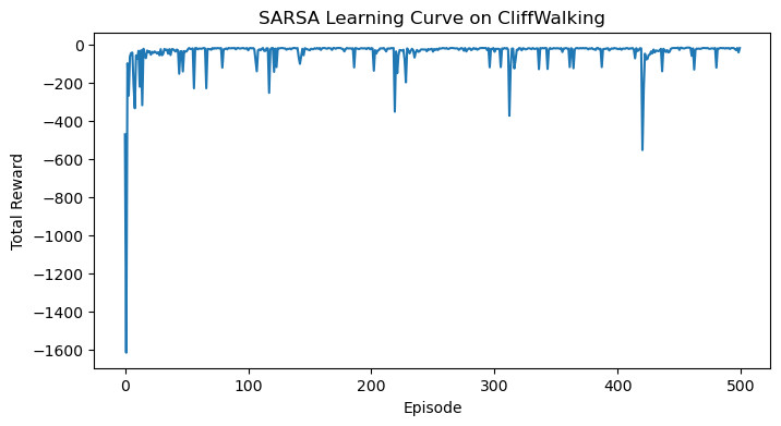
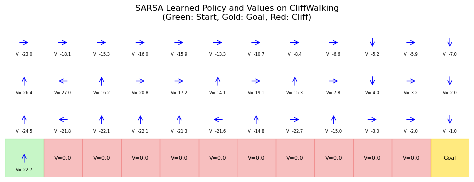
This learns a safe path along the top, avoiding the cliff.

13.6.4 Off-Policy TD Control: Q-Learning

Q-Learning is an off-policy TD control method that learns the optimal \( Q^*(s,a) \) while exploring with a separate behavior policy (e.g., ε-greedy). It uses importance sampling implicitly via the max operator, allowing data reuse and decoupling exploration from the target greedy policy.

Algorithm:

1. Initialize \(Q(s, a) = 0 \).

2. For each step:

   • From \( s \), choose \( a \) from behavior policy.

   • Observe \( r, s' \).

   • Update: \( Q(s, a) \leftarrow Q(s, a) + \alpha [r + \gamma \max_{a'} Q(s', a') - Q(s, a)] \).

3. The max assumes the optimal policy, converging to \( Q^* \)regardless of behavior (as long as all pairs are visited infinitely). The max assumes the optimal policy, converging to \( Q^* \) regardless of behavior (as long as all pairs are visited infinitely).

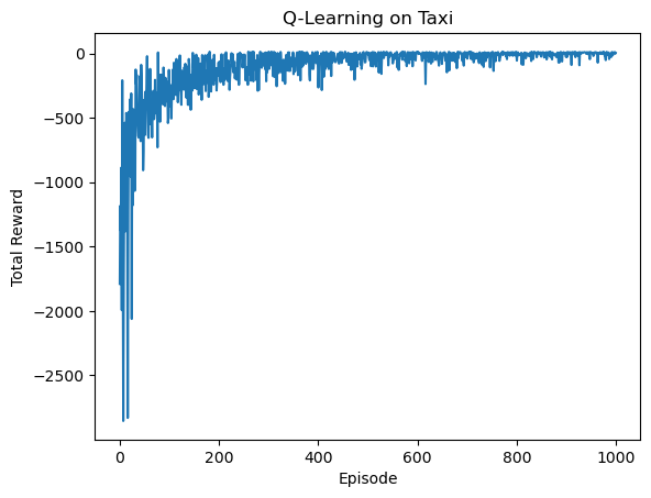
Importance sampling corrects for policy differences in off-policy learning generally, but Q-Learning avoids explicit ratios by targeting the optimal. In space, it’s ideal for sim-based training with aggressive exploration, transferring to conservative real policies. Below is a Python example of tabular Q-Learning on Gymnasium’s Taxi environment (5x5 grid; 4 passenger locations, 4 destinations; actions: move N/S/E/W, pickup/dropoff).

import gymnasium as gym
import numpy as np

env = gym.make('Taxi-v3')
num_episodes = 1000
alpha = 0.1
gamma = 0.99
epsilon = 0.1

# Q-table: 500 states, 6 actions
Q = np.zeros((env.observation_space.n, env.action_space.n))

episode_rewards = []
for episode in range(num_episodes):
    state, _ = env.reset()
    total_reward = 0
    done = False
    while not done:
        action = np.argmax(Q[state]) if np.random.rand() > epsilon else env.action_space.sample()
        next_state, reward, done, _, _ = env.step(action)
        Q[state, action] += alpha * (reward + gamma * np.max(Q[next_state]) - Q[state, action])
        state = next_state
        total_reward += reward
    episode_rewards.append(total_reward)

# Plot
import matplotlib.pyplot as plt
plt.plot(episode_rewards)
plt.xlabel('Episode')
plt.ylabel('Total Reward')
plt.title('Q-Learning on Taxi')
plt.show()

# Policy
policy = np.argmax(Q, axis=1)
print("Optimal Policy Snippet (first 10 states):", policy[:10])

Optimal Policy Snippet (first 10 states): [0 4 4 4 2 0 1 1 0 2]

This learns efficient taxi navigation, with rewards improving to ~8-10 per episode.

13.7 Function Approximation and Deep Reinforcement Learning

Tabular methods like those in previous sections work well for small, discrete state-action spaces but fail in high-dimensional or continuous environments common in engineering, such as spacecraft dynamics with continuous states (position, velocity, attitude). Function approximation addresses this by parameterizing value functions or policies with models like linear regressors or neural networks, enabling generalization across similar states. This scales RL to real-world problems, evolving from simple linear approximations (e.g., tile coding) to deep neural networks that learn hierarchical features from raw inputs like sensor data. In space engineering, this allows handling complex, non-linear systems like orbital perturbations without exhaustive tabulation.

13.7.1 Need for Function Approximation

The curse of dimensionality plagues tabular RL: As state dimensions grow (e.g., 6-DOF spacecraft pose plus velocities), the number of states explodes exponentially, making storage and exploration infeasible. For instance, discretizing each dimension into 10 bins yields \( 10^d \) states for \( d \) dimensions—unmanageable for \( d > 10 \).

Function approximation mitigates this by representing values as parameterized functions, e.g., \( \hat{V}(s; \theta) \approx V^\pi(s) \) or \( \hat{Q}(s,a; \theta) \approx Q^\pi(s,a) \), where \( \theta \) are weights updated via gradient descent on errors like TD residuals. Linear approximators (e.g., \( \hat{V}(s) = \theta^\top \phi(s) \), with features \( \phi \)) offer guarantees in some cases, but non-linear models like neural nets handle complex mappings. This enables RL in continuous spaces, crucial for engineering tasks like optimal control under uncertainty.

13.7.2 Deep Q-Networks (DQN)

Deep Q-Networks (DQN) extend Q-learning to high-dimensional inputs using deep neural networks as Q-approximators, \( Q(s,a; \theta) \). The architecture typically includes convolutional layers for image inputs (e.g., from cameras) or fully connected layers for vector states, outputting Q-values for each action.

Key innovations include experience replay: A buffer stores transitions \( (s, a, r, s') \), sampled in mini-batches to break correlations and stabilize training. Target networks decouple updates: A separate network \( Q(s',a'; \theta^-) \) computes targets, updated slowly (e.g., soft: \( \theta^- \leftarrow \tau \theta + (1-\tau) \theta^- \)) to reduce oscillations. DQN optimizes via SGD on the loss \( \mathcal{L} = [r + \gamma \max_{a'} Q(s',a'; \theta^-) - Q(s,a; \theta)]^2 \), with ε-greedy exploration.

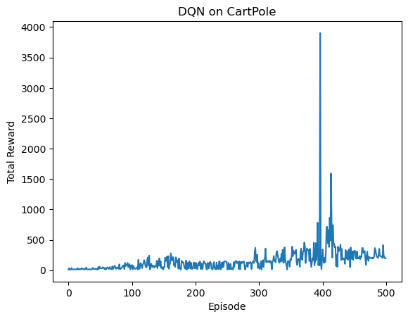
Example: DQN on CartPole

Below is a Python example of a simple DQN using PyTorch on Gymnasium’s CartPole-v1 (continuous state: cart position/velocity, pole angle/rate; discrete actions: left/right). It trains an agent to balance the pole.

import gymnasium as gym
import numpy as np
import torch
import torch.nn as nn
import torch.optim as optim
from collections import deque
import random
import matplotlib.pyplot as plt
from matplotlib import animation
from IPython.display import HTML  # For displaying animation in Jupyter

# Hyperparameters
env = gym.make('CartPole-v1', render_mode='rgb_array')  # Enable rgb_array for frames
state_dim = env.observation_space.shape[0]  # 4
action_dim = env.action_space.n  # 2
hidden_dim = 64
gamma = 0.99
epsilon_start = 1.0
epsilon_end = 0.01
epsilon_decay = 0.995
batch_size = 64
lr = 0.001
target_update = 10  # episodes
buffer_size = 10000
num_episodes = 500

# Neural Network
class DQN(nn.Module):
    def __init__(self, state_dim, action_dim, hidden_dim):
        super(DQN, self).__init__()
        self.fc1 = nn.Linear(state_dim, hidden_dim)
        self.fc2 = nn.Linear(hidden_dim, hidden_dim)
        self.out = nn.Linear(hidden_dim, action_dim)

    def forward(self, x):
        x = torch.relu(self.fc1(x))
        x = torch.relu(self.fc2(x))
        return self.out(x)

# Replay Buffer
replay_buffer = deque(maxlen=buffer_size)

# Networks
policy_net = DQN(state_dim, action_dim, hidden_dim)
target_net = DQN(state_dim, action_dim, hidden_dim)
target_net.load_state_dict(policy_net.state_dict())
optimizer = optim.Adam(policy_net.parameters(), lr=lr)
criterion = nn.MSELoss()

def select_action(state, epsilon):
    if random.random() < epsilon:
        return env.action_space.sample()
    state = torch.FloatTensor(state).unsqueeze(0)
    with torch.no_grad():
        q_values = policy_net(state)
    return q_values.argmax().item()

# Training
episode_rewards = []
epsilon = epsilon_start
for episode in range(num_episodes):
    state, _ = env.reset()
    total_reward = 0
    done = False
    while not done:
        action = select_action(state, epsilon)
        next_state, reward, done, _, _ = env.step(action)
        total_reward += reward
        replay_buffer.append((state, action, reward, next_state, done))
        state = next_state

        if len(replay_buffer) > batch_size:
            batch = random.sample(replay_buffer, batch_size)
            states, actions, rewards, next_states, dones = zip(*batch)
            states = torch.FloatTensor(np.array(states))
            actions = torch.LongTensor(actions).unsqueeze(1)
            rewards = torch.FloatTensor(rewards)
            next_states = torch.FloatTensor(np.array(next_states))
            dones = torch.FloatTensor(dones)

            q_values = policy_net(states).gather(1, actions).squeeze()
            with torch.no_grad():
                next_q_values = target_net(next_states).max(1)[0]
            targets = rewards + gamma * next_q_values * (1 - dones)

            loss = criterion(q_values, targets)
            optimizer.zero_grad()
            loss.backward()
            optimizer.step()

    episode_rewards.append(total_reward)
    epsilon = max(epsilon_end, epsilon * epsilon_decay)

    if episode % target_update == 0:
        target_net.load_state_dict(policy_net.state_dict())

# Plot rewards
plt.plot(episode_rewards)
plt.xlabel('Episode')
plt.ylabel('Total Reward')
plt.title('DQN on CartPole')
plt.show()

# Evaluation with visualization
def evaluate_and_visualize(num_steps=200):
    state, _ = env.reset()
    frames = []  # Collect RGB frames
    done = False
    step = 0
    while not done and step < num_steps:
        frame = env.render()  # Get RGB array
        frames.append(frame)
        action = select_action(state, 0)  # Greedy
        state, _, done, _, _ = env.step(action)
        step += 1
    env.close()

    # Animate frames
    fig = plt.figure()
    img = plt.imshow(frames[0])
    def animate(i):
        img.set_array(frames[i])
        return [img]
    anim = animation.FuncAnimation(fig, animate, frames=len(frames), interval=50)
    plt.close()  # Close to prevent static display
    return anim

# Display animation in Jupyter (requires %matplotlib inline or notebook)
anim = evaluate_and_visualize()
HTML(anim.to_jshtml())

/home/stefan_endres/.anaconda3/envs/comp_eng/lib/python3.12/site-packages/pygame/pkgdata.py:25: UserWarning: pkg_resources is deprecated as an API. See https://setuptools.pypa.io/en/latest/pkg_resources.html. The pkg_resources package is slated for removal as early as 2025-11-30. Refrain from using this package or pin to Setuptools<81.
  from pkg_resources import resource_stream, resource_exists

Once Loop Reflect

13.7.3 Stability and Extensions

DQN’s basic form can suffer from overestimation bias (max operator amplifies noise) and instability. Double DQN addresses bias by decoupling action selection and evaluation: Target uses policy net for argmax, target net for value: reducing overoptimism in uncertain space environments.

Dueling DQN factorizes Q into state-value \( V(s) \) and advantage \( A(s,a) \): \( Q(s,a) = V(s) + (A(s,a) - \frac{1}{|A|} \sum_{a'} A(s,a')) \), with separate streams in the network. This improves learning by isolating state quality from action benefits, aiding tasks like multi-axis satellite control with shared state values. These extensions enhance robustness for engineering deployments.

13.8 Policy Gradient Methods and Actor-Critic

Policy gradient methods shift from value-based approaches (like Q-learning) to direct policy optimization, parameterizing the policy \( \pi_\theta(a|s) \) (e.g., as a neural network with weights \( \theta \)) and updating \( \theta \) to maximize expected returns. This is advantageous in continuous action spaces, common in engineering, where discretizing actions is impractical (e.g., variable thrust in satellite control). The foundational REINFORCE algorithm uses Monte-Carlo estimates of gradients, but suffers from high variance due to full-episode sampling. Baselines (e.g., subtracting a state-value estimate) reduce variance without introducing bias, improving stability. Actor-critic methods combine policy gradients (the “actor”) with value estimation (the “critic”), enabling bootstrapping for lower variance and faster learning: key for real-time adaptation in space systems like non-linear orbit maneuvers under perturbations.

In the course nomenclature, the state \( s \) aligns with the dynamic state vector \( \mathbf{y}(t) \) (e.g., position and velocity), while actions \( a \) correspond to control inputs \( \mathbf{u} \) (e.g., thrust), and the dynamics relate to \( \dot{\mathbf{y}} = \mathbf{f}(\mathbf{y}, \mathbf{u}) \), with parameters \( \mathbf{p} \) capturing uncertainties like drag.

13.8.1 Policy Gradient Theorem

The policy gradient theorem provides a mathematical foundation for directly computing gradients of the performance objective \( J(\theta) = \mathbb{E}_\pi [G_0] \), the expected return under policy \( \pi_\theta \).

At a high level, the derivation starts from the MDP framework, expressing \( J(\theta) \) via the stationary distribution \( d^\pi(s) \) (probability of visiting \( s \) under \( \pi \)): \( J(\theta) = \sum_s d^\pi(s) \sum_a \pi_\theta(a|s) Q^\pi(s,a). \)

Differentiating with respect to \( \theta \) (using the log-trick \( \nabla_\theta \pi = \pi \nabla_\theta \log \pi \)) yields:

\( \nabla_\theta J(\theta) = \mathbb{E}_\pi \left[ \nabla_\theta \log \pi_\theta(a|s) Q^\pi(s,a) \right], \)

where the expectation is over states and actions sampled from trajectories under \( \pi_\theta \). Replacing \( Q^\pi \) with sampled returns \( G_t \) (Monte-Carlo) or advantages (to reduce variance) enables stochastic gradient ascent: \( \theta \leftarrow \theta + \alpha \nabla_\theta J(\theta) \). This theorem ensures unbiased gradients, even in stochastic policies, making it suitable for fine-grained control in engineering, like optimizing probabilistic thrust profiles for fuel efficiency.

Relating to course nomenclature, \( s \) here is akin to \( \mathbf{y} \), \( a \) to \( \mathbf{u} \), and the objective ties to optimizing over feasible sets \( \mathcal{Y} \) and parameters \( \mathbf{p} \).

13.8.2 REINFORCE Algorithm

REINFORCE (REward Increment = Nonnegative Factor times Offset Reinforcement and Characteristic Eligibility) is a Monte-Carlo policy gradient method that samples full episodes to estimate \( \nabla_\theta J(\theta) \), updating the policy via: \( \theta \leftarrow \theta + \alpha G_t \nabla_\theta \log \pi_\theta(a_t | s_t), \)

summing over timesteps \( t \) (with discounting). It directly optimizes stochastic policies, ideal for exploration in continuous spaces.

However, variance issues arise from noisy return estimates \( G_t \), especially in long-horizon tasks—leading to slow convergence or instability. Baselines (e.g., subtracting \( V(s_t) \)) mitigate this: \( G_t - V(s_t) \), centering gradients around zero without bias. In space engineering, REINFORCE suits episodic simulations like trajectory optimization, but variance challenges real-time use.

Below is a Python example of vanilla REINFORCE (with baseline) using PyTorch on Gymnasium’s Pendulum-v1 (continuous action: torque \( [-2,2] \); state: angle/velocity; goal: upright balance). The state relates to \( \mathbf{y} \), action to scalar \( u \).

import gymnasium as gym
import numpy as np
import torch
import torch.nn as nn
import torch.optim as optim
import torch.nn.functional as F
from torch.distributions import Normal
import matplotlib.pyplot as plt

# Set seed for reproducibility
seed = 42
torch.manual_seed(seed)
np.random.seed(seed)
env = gym.make('Pendulum-v1')
env.reset(seed=seed)

# Hyperparameters (further tuned)
state_dim = env.observation_space.shape[0]  # 3
action_dim = 1  # Continuous torque
hidden_dim = 128
lr_actor = 3e-4
lr_critic = 1e-3
gamma = 0.99
num_episodes = 3000  # Increased further
max_steps = 300
entropy_beta = 0.01
clip_grad_norm = 1.0  # New: Gradient clipping value
num_envs = 4  # New: Multi-env rollouts for variance reduction

# Policy Network (Actor)
class PolicyNet(nn.Module):
    def __init__(self, state_dim, action_dim, hidden_dim):
        super(PolicyNet, self).__init__()
        self.fc1 = nn.Linear(state_dim, hidden_dim)
        self.fc2 = nn.Linear(hidden_dim, hidden_dim)
        self.fc_mu = nn.Linear(hidden_dim, action_dim)
        self.fc_sigma = nn.Linear(hidden_dim, action_dim)

    def forward(self, x):
        x = torch.relu(self.fc1(x))
        x = torch.relu(self.fc2(x))
        mu = 2 * torch.tanh(self.fc_mu(x))  # Scale to [-2,2]
        sigma = F.softplus(self.fc_sigma(x)) + 1e-5
        return mu, sigma

    def sample(self, state):
        mu, sigma = self(state)
        dist = Normal(mu, sigma)
        action = dist.sample()
        log_prob = dist.log_prob(action)
        entropy = dist.entropy()
        return action.item(), log_prob, entropy

# Value Network (Baseline)
class ValueNet(nn.Module):
    def __init__(self, state_dim, hidden_dim):
        super(ValueNet, self).__init__()
        self.fc1 = nn.Linear(state_dim, hidden_dim)
        self.fc2 = nn.Linear(hidden_dim, hidden_dim)
        self.fc3 = nn.Linear(hidden_dim, 1)

    def forward(self, x):
        x = torch.relu(self.fc1(x))
        x = torch.relu(self.fc2(x))
        return self.fc3(x)

# Initialize
policy_net = PolicyNet(state_dim, action_dim, hidden_dim)
value_net = ValueNet(state_dim, hidden_dim)
actor_optim = optim.AdamW(policy_net.parameters(), lr=lr_actor)
critic_optim = optim.AdamW(value_net.parameters(), lr=lr_critic)
criterion = nn.MSELoss()

# Training with multi-env rollouts
episode_rewards = []
actor_losses = []
critic_losses = []
avg_entropies = []
for episode in range(num_episodes):
    # Collect multiple trajectories
    all_log_probs = []
    all_rewards = []
    all_values = []
    all_entropies = []
    batch_rewards = 0
    for _ in range(num_envs):
        state, _ = env.reset()
        log_probs = []
        rewards = []
        values = []
        entropies = []
        done = False
        step = 0
        while not done and step < max_steps:
            state_tensor = torch.FloatTensor(state)
            action, log_prob, entropy = policy_net.sample(state_tensor)
            value = value_net(state_tensor)
            next_state, reward, done, _, _ = env.step([action])

            log_probs.append(log_prob)
            rewards.append(reward)
            values.append(value)
            entropies.append(entropy)

            state = next_state
            step += 1

        all_log_probs.extend(log_probs)
        all_rewards.extend(rewards)
        all_values.extend(values)
        all_entropies.extend(entropies)
        batch_rewards += sum(rewards)

    # Compute returns and advantages (across batch)
    returns = []
    G = 0
    for r in reversed(all_rewards):
        G = r + gamma * G
        returns.insert(0, G)
    returns = torch.FloatTensor(returns)
    values = torch.cat(all_values).squeeze()
    advantages = returns - values.detach()
    advantages = (advantages - advantages.mean()) / (advantages.std() + 1e-8)  # Normalize

    # Actor loss with entropy
    actor_loss = -torch.sum(torch.stack(all_log_probs) * advantages) - entropy_beta * torch.mean(torch.stack(all_entropies))
    actor_optim.zero_grad()
    actor_loss.backward()
    torch.nn.utils.clip_grad_norm_(policy_net.parameters(), clip_grad_norm)  # Clip gradients
    actor_optim.step()

    # Critic loss
    critic_loss = criterion(values, returns)
    critic_optim.zero_grad()
    critic_loss.backward()
    torch.nn.utils.clip_grad_norm_(value_net.parameters(), clip_grad_norm)  # Clip gradients
    critic_optim.step()

    episode_rewards.append(batch_rewards / num_envs)  # Average per env
    actor_losses.append(actor_loss.item())
    critic_losses.append(critic_loss.item())
    avg_entropies.append(torch.mean(torch.stack(all_entropies)).item())

    if episode % 100 == 0:
        print(f"Episode {episode}: Avg Reward = {episode_rewards[-1]:.2f}, Avg Entropy = {avg_entropies[-1]:.2f}")

# Plots
fig, axs = plt.subplots(2, 2, figsize=(12, 8))
axs[0, 0].plot(episode_rewards); axs[0, 0].set_title('Episode Rewards')
axs[0, 1].plot(avg_entropies); axs[0, 1].set_title('Average Entropy')
axs[1, 0].plot(actor_losses); axs[1, 0].set_title('Actor Losses')
axs[1, 1].plot(critic_losses); axs[1, 1].set_title('Critic Losses')
plt.tight_layout()
plt.show()

Episode 0: Avg Reward = -1907.92, Avg Entropy = 0.94
Episode 100: Avg Reward = -1878.24, Avg Entropy = 2.34
Episode 200: Avg Reward = -1814.04, Avg Entropy = 3.01
Episode 300: Avg Reward = -1803.52, Avg Entropy = 3.61
Episode 400: Avg Reward = -2074.49, Avg Entropy = 3.96
Episode 500: Avg Reward = -1751.90, Avg Entropy = 4.59
Episode 600: Avg Reward = -1849.64, Avg Entropy = 4.91
Episode 700: Avg Reward = -1866.67, Avg Entropy = 5.18
Episode 800: Avg Reward = -1985.54, Avg Entropy = 5.36
Episode 900: Avg Reward = -1779.81, Avg Entropy = 5.73
Episode 1000: Avg Reward = -1916.43, Avg Entropy = 5.96
Episode 1100: Avg Reward = -2087.99, Avg Entropy = 6.04
Episode 1200: Avg Reward = -1835.01, Avg Entropy = 6.33
Episode 1300: Avg Reward = -1642.47, Avg Entropy = 6.56
Episode 1400: Avg Reward = -1896.86, Avg Entropy = 6.65
Episode 1500: Avg Reward = -1826.53, Avg Entropy = 6.77
Episode 1600: Avg Reward = -2113.59, Avg Entropy = 6.88
Episode 1700: Avg Reward = -1858.91, Avg Entropy = 7.04
Episode 1800: Avg Reward = -1759.09, Avg Entropy = 7.27
Episode 1900: Avg Reward = -1654.58, Avg Entropy = 7.40
Episode 2000: Avg Reward = -1954.49, Avg Entropy = 7.44
Episode 2100: Avg Reward = -1880.90, Avg Entropy = 7.61
Episode 2200: Avg Reward = -1992.86, Avg Entropy = 7.69
Episode 2300: Avg Reward = -1917.06, Avg Entropy = 7.81
Episode 2400: Avg Reward = -1775.28, Avg Entropy = 7.99
Episode 2500: Avg Reward = -1888.56, Avg Entropy = 8.04
Episode 2600: Avg Reward = -2056.87, Avg Entropy = 8.08
Episode 2700: Avg Reward = -1673.15, Avg Entropy = 8.21
Episode 2800: Avg Reward = -1497.19, Avg Entropy = 8.38
Episode 2900: Avg Reward = -1802.42, Avg Entropy = 8.42

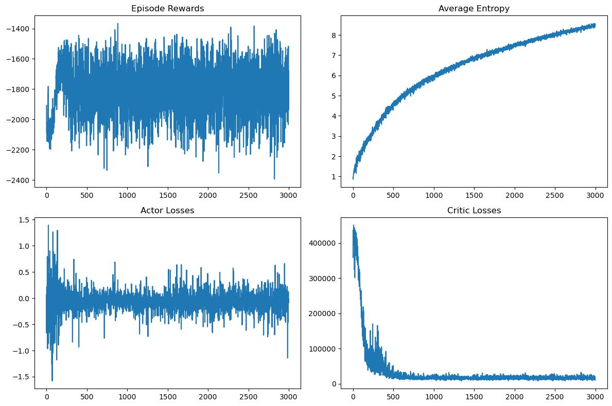
from stable_baselines3 import PPO
from stable_baselines3.common.env_util import make_vec_env
import gymnasium as gym
import matplotlib.pyplot as plt

# Hyperparameters
env_id = "Pendulum-v1"
num_envs = 4
vec_env = make_vec_env(env_id, n_envs=num_envs)

model = PPO("MlpPolicy", vec_env, verbose=1, n_steps=2048, batch_size=64, n_epochs=10, learning_rate=3e-4)

# Training
model.learn(total_timesteps=300000)  # ~3000 effective episodes

# Evaluation
episode_rewards = []
for episode in range(10):
    obs = vec_env.reset()
    done = [False] * num_envs
    total_reward = [0] * num_envs
    while not all(done):
        action, _ = model.predict(obs, deterministic=True)
        obs, reward, done, _ = vec_env.step(action)
        for i in range(num_envs):
            total_reward[i] += reward[i]
    episode_rewards.append(np.mean(total_reward))

print("Mean Eval Reward:", np.mean(episode_rewards))

# Plot (for training, use tensorboard if set up)
plt.plot(episode_rewards)  # Eval only
plt.title('PPO Eval Rewards on Pendulum')
plt.show()

Using cuda device

/home/stefan_endres/.anaconda3/envs/comp_eng/lib/python3.12/site-packages/stable_baselines3/common/on_policy_algorithm.py:150: UserWarning: You are trying to run PPO on the GPU, but it is primarily intended to run on the CPU when not using a CNN policy (you are using ActorCriticPolicy which should be a MlpPolicy). See https://github.com/DLR-RM/stable-baselines3/issues/1245 for more info. You can pass `device='cpu'` or `export CUDA_VISIBLE_DEVICES=` to force using the CPU.Note: The model will train, but the GPU utilization will be poor and the training might take longer than on CPU.
  warnings.warn(

---------------------------------
| rollout/           |          |
|    ep_len_mean     | 200      |
|    ep_rew_mean     | -1.2e+03 |
| time/              |          |
|    fps             | 8117     |
|    iterations      | 1        |
|    time_elapsed    | 1        |
|    total_timesteps | 8192     |
---------------------------------
-----------------------------------------
| rollout/                |             |
|    ep_len_mean          | 200         |
|    ep_rew_mean          | -1.17e+03   |
| time/                   |             |
|    fps                  | 4113        |
|    iterations           | 2           |
|    time_elapsed         | 3           |
|    total_timesteps      | 16384       |
| train/                  |             |
|    approx_kl            | 0.004302967 |
|    clip_fraction        | 0.028       |
|    clip_range           | 0.2         |
|    entropy_loss         | -1.41       |
|    explained_variance   | 0.0013      |
|    learning_rate        | 0.0003      |
|    loss                 | 2.01e+03    |
|    n_updates            | 10          |
|    policy_gradient_loss | -0.00192    |
|    std                  | 0.981       |
|    value_loss           | 6.8e+03     |
-----------------------------------------
------------------------------------------
| rollout/                |              |
|    ep_len_mean          | 200          |
|    ep_rew_mean          | -1.17e+03    |
| time/                   |              |
|    fps                  | 3542         |
|    iterations           | 3            |
|    time_elapsed         | 6            |
|    total_timesteps      | 24576        |
| train/                  |              |
|    approx_kl            | 0.0036599482 |
|    clip_fraction        | 0.0126       |
|    clip_range           | 0.2          |
|    entropy_loss         | -1.38        |
|    explained_variance   | 0.0139       |
|    learning_rate        | 0.0003       |
|    loss                 | 2.17e+03     |
|    n_updates            | 20           |
|    policy_gradient_loss | -0.00138     |
|    std                  | 0.951        |
|    value_loss           | 5.83e+03     |
------------------------------------------
-----------------------------------------
| rollout/                |             |
|    ep_len_mean          | 200         |
|    ep_rew_mean          | -1.16e+03   |
| time/                   |             |
|    fps                  | 3346        |
|    iterations           | 4           |
|    time_elapsed         | 9           |
|    total_timesteps      | 32768       |
| train/                  |             |
|    approx_kl            | 0.002959379 |
|    clip_fraction        | 0.0207      |
|    clip_range           | 0.2         |
|    entropy_loss         | -1.36       |
|    explained_variance   | 0.0011      |
|    learning_rate        | 0.0003      |
|    loss                 | 1.74e+03    |
|    n_updates            | 30          |
|    policy_gradient_loss | -0.00185    |
|    std                  | 0.936       |
|    value_loss           | 6.05e+03    |
-----------------------------------------
------------------------------------------
| rollout/                |              |
|    ep_len_mean          | 200          |
|    ep_rew_mean          | -1.14e+03    |
| time/                   |              |
|    fps                  | 3235         |
|    iterations           | 5            |
|    time_elapsed         | 12           |
|    total_timesteps      | 40960        |
| train/                  |              |
|    approx_kl            | 0.0033616915 |
|    clip_fraction        | 0.0245       |
|    clip_range           | 0.2          |
|    entropy_loss         | -1.35        |
|    explained_variance   | 0.000446     |
|    learning_rate        | 0.0003       |
|    loss                 | 1.74e+03     |
|    n_updates            | 40           |
|    policy_gradient_loss | -0.00144     |
|    std                  | 0.937        |
|    value_loss           | 4.74e+03     |
------------------------------------------
------------------------------------------
| rollout/                |              |
|    ep_len_mean          | 200          |
|    ep_rew_mean          | -1.09e+03    |
| time/                   |              |
|    fps                  | 3165         |
|    iterations           | 6            |
|    time_elapsed         | 15           |
|    total_timesteps      | 49152        |
| train/                  |              |
|    approx_kl            | 0.0030833608 |
|    clip_fraction        | 0.0175       |
|    clip_range           | 0.2          |
|    entropy_loss         | -1.35        |
|    explained_variance   | 0.000132     |
|    learning_rate        | 0.0003       |
|    loss                 | 1.62e+03     |
|    n_updates            | 50           |
|    policy_gradient_loss | -0.0017      |
|    std                  | 0.937        |
|    value_loss           | 3.99e+03     |
------------------------------------------
------------------------------------------
| rollout/                |              |
|    ep_len_mean          | 200          |
|    ep_rew_mean          | -1.12e+03    |
| time/                   |              |
|    fps                  | 3117         |
|    iterations           | 7            |
|    time_elapsed         | 18           |
|    total_timesteps      | 57344        |
| train/                  |              |
|    approx_kl            | 0.0023397445 |
|    clip_fraction        | 0.0194       |
|    clip_range           | 0.2          |
|    entropy_loss         | -1.35        |
|    explained_variance   | 6.8e-05      |
|    learning_rate        | 0.0003       |
|    loss                 | 1.1e+03      |
|    n_updates            | 60           |
|    policy_gradient_loss | -0.00154     |
|    std                  | 0.937        |
|    value_loss           | 3.36e+03     |
------------------------------------------
-----------------------------------------
| rollout/                |             |
|    ep_len_mean          | 200         |
|    ep_rew_mean          | -1.13e+03   |
| time/                   |             |
|    fps                  | 3081        |
|    iterations           | 8           |
|    time_elapsed         | 21          |
|    total_timesteps      | 65536       |
| train/                  |             |
|    approx_kl            | 0.002641587 |
|    clip_fraction        | 0.0068      |
|    clip_range           | 0.2         |
|    entropy_loss         | -1.34       |
|    explained_variance   | 2.62e-05    |
|    learning_rate        | 0.0003      |
|    loss                 | 1.2e+03     |
|    n_updates            | 70          |
|    policy_gradient_loss | -0.000407   |
|    std                  | 0.916       |
|    value_loss           | 3.7e+03     |
-----------------------------------------
------------------------------------------
| rollout/                |              |
|    ep_len_mean          | 200          |
|    ep_rew_mean          | -1.12e+03    |
| time/                   |              |
|    fps                  | 3055         |
|    iterations           | 9            |
|    time_elapsed         | 24           |
|    total_timesteps      | 73728        |
| train/                  |              |
|    approx_kl            | 0.0055417214 |
|    clip_fraction        | 0.0322       |
|    clip_range           | 0.2          |
|    entropy_loss         | -1.3         |
|    explained_variance   | 2.29e-05     |
|    learning_rate        | 0.0003       |
|    loss                 | 851          |
|    n_updates            | 80           |
|    policy_gradient_loss | -0.00221     |
|    std                  | 0.876        |
|    value_loss           | 2.87e+03     |
------------------------------------------
------------------------------------------
| rollout/                |              |
|    ep_len_mean          | 200          |
|    ep_rew_mean          | -1.1e+03     |
| time/                   |              |
|    fps                  | 3034         |
|    iterations           | 10           |
|    time_elapsed         | 27           |
|    total_timesteps      | 81920        |
| train/                  |              |
|    approx_kl            | 0.0036573368 |
|    clip_fraction        | 0.0244       |
|    clip_range           | 0.2          |
|    entropy_loss         | -1.28        |
|    explained_variance   | 1.31e-05     |
|    learning_rate        | 0.0003       |
|    loss                 | 872          |
|    n_updates            | 90           |
|    policy_gradient_loss | -0.00166     |
|    std                  | 0.87         |
|    value_loss           | 2.41e+03     |
------------------------------------------
------------------------------------------
| rollout/                |              |
|    ep_len_mean          | 200          |
|    ep_rew_mean          | -1.13e+03    |
| time/                   |              |
|    fps                  | 3015         |
|    iterations           | 11           |
|    time_elapsed         | 29           |
|    total_timesteps      | 90112        |
| train/                  |              |
|    approx_kl            | 0.0026808681 |
|    clip_fraction        | 0.0181       |
|    clip_range           | 0.2          |
|    entropy_loss         | -1.28        |
|    explained_variance   | 8.05e-06     |
|    learning_rate        | 0.0003       |
|    loss                 | 573          |
|    n_updates            | 100          |
|    policy_gradient_loss | -0.000874    |
|    std                  | 0.867        |
|    value_loss           | 2.21e+03     |
------------------------------------------
------------------------------------------
| rollout/                |              |
|    ep_len_mean          | 200          |
|    ep_rew_mean          | -1.11e+03    |
| time/                   |              |
|    fps                  | 3001         |
|    iterations           | 12           |
|    time_elapsed         | 32           |
|    total_timesteps      | 98304        |
| train/                  |              |
|    approx_kl            | 0.0044386974 |
|    clip_fraction        | 0.0295       |
|    clip_range           | 0.2          |
|    entropy_loss         | -1.27        |
|    explained_variance   | 6.2e-06      |
|    learning_rate        | 0.0003       |
|    loss                 | 527          |
|    n_updates            | 110          |
|    policy_gradient_loss | -0.00221     |
|    std                  | 0.862        |
|    value_loss           | 1.93e+03     |
------------------------------------------
-----------------------------------------
| rollout/                |             |
|    ep_len_mean          | 200         |
|    ep_rew_mean          | -1.09e+03   |
| time/                   |             |
|    fps                  | 2989        |
|    iterations           | 13          |
|    time_elapsed         | 35          |
|    total_timesteps      | 106496      |
| train/                  |             |
|    approx_kl            | 0.003546575 |
|    clip_fraction        | 0.0276      |
|    clip_range           | 0.2         |
|    entropy_loss         | -1.28       |
|    explained_variance   | 5.96e-06    |
|    learning_rate        | 0.0003      |
|    loss                 | 471         |
|    n_updates            | 120         |
|    policy_gradient_loss | -0.0011     |
|    std                  | 0.876       |
|    value_loss           | 1.43e+03    |
-----------------------------------------
------------------------------------------
| rollout/                |              |
|    ep_len_mean          | 200          |
|    ep_rew_mean          | -1.12e+03    |
| time/                   |              |
|    fps                  | 2980         |
|    iterations           | 14           |
|    time_elapsed         | 38           |
|    total_timesteps      | 114688       |
| train/                  |              |
|    approx_kl            | 0.0048263245 |
|    clip_fraction        | 0.0415       |
|    clip_range           | 0.2          |
|    entropy_loss         | -1.29        |
|    explained_variance   | 5.07e-06     |
|    learning_rate        | 0.0003       |
|    loss                 | 458          |
|    n_updates            | 130          |
|    policy_gradient_loss | -0.00287     |
|    std                  | 0.877        |
|    value_loss           | 1.42e+03     |
------------------------------------------
----------------------------------------
| rollout/                |            |
|    ep_len_mean          | 200        |
|    ep_rew_mean          | -1.14e+03  |
| time/                   |            |
|    fps                  | 2971       |
|    iterations           | 15         |
|    time_elapsed         | 41         |
|    total_timesteps      | 122880     |
| train/                  |            |
|    approx_kl            | 0.00398001 |
|    clip_fraction        | 0.0246     |
|    clip_range           | 0.2        |
|    entropy_loss         | -1.27      |
|    explained_variance   | 0.0016     |
|    learning_rate        | 0.0003     |
|    loss                 | 488        |
|    n_updates            | 140        |
|    policy_gradient_loss | -0.00156   |
|    std                  | 0.848      |
|    value_loss           | 1.36e+03   |
----------------------------------------
------------------------------------------
| rollout/                |              |
|    ep_len_mean          | 200          |
|    ep_rew_mean          | -1.17e+03    |
| time/                   |              |
|    fps                  | 2964         |
|    iterations           | 16           |
|    time_elapsed         | 44           |
|    total_timesteps      | 131072       |
| train/                  |              |
|    approx_kl            | 0.0035657794 |
|    clip_fraction        | 0.0338       |
|    clip_range           | 0.2          |
|    entropy_loss         | -1.26        |
|    explained_variance   | 0.174        |
|    learning_rate        | 0.0003       |
|    loss                 | 218          |
|    n_updates            | 150          |
|    policy_gradient_loss | -0.00201     |
|    std                  | 0.855        |
|    value_loss           | 1.11e+03     |
------------------------------------------
------------------------------------------
| rollout/                |              |
|    ep_len_mean          | 200          |
|    ep_rew_mean          | -1.16e+03    |
| time/                   |              |
|    fps                  | 2957         |
|    iterations           | 17           |
|    time_elapsed         | 47           |
|    total_timesteps      | 139264       |
| train/                  |              |
|    approx_kl            | 0.0071209697 |
|    clip_fraction        | 0.0614       |
|    clip_range           | 0.2          |
|    entropy_loss         | -1.24        |
|    explained_variance   | 0.457        |
|    learning_rate        | 0.0003       |
|    loss                 | 273          |
|    n_updates            | 160          |
|    policy_gradient_loss | -0.00452     |
|    std                  | 0.826        |
|    value_loss           | 978          |
------------------------------------------
------------------------------------------
| rollout/                |              |
|    ep_len_mean          | 200          |
|    ep_rew_mean          | -1.12e+03    |
| time/                   |              |
|    fps                  | 2952         |
|    iterations           | 18           |
|    time_elapsed         | 49           |
|    total_timesteps      | 147456       |
| train/                  |              |
|    approx_kl            | 0.0042206696 |
|    clip_fraction        | 0.0518       |
|    clip_range           | 0.2          |
|    entropy_loss         | -1.22        |
|    explained_variance   | 0.666        |
|    learning_rate        | 0.0003       |
|    loss                 | 151          |
|    n_updates            | 170          |
|    policy_gradient_loss | -0.00333     |
|    std                  | 0.819        |
|    value_loss           | 556          |
------------------------------------------
-----------------------------------------
| rollout/                |             |
|    ep_len_mean          | 200         |
|    ep_rew_mean          | -1.05e+03   |
| time/                   |             |
|    fps                  | 2947        |
|    iterations           | 19          |
|    time_elapsed         | 52          |
|    total_timesteps      | 155648      |
| train/                  |             |
|    approx_kl            | 0.005966984 |
|    clip_fraction        | 0.061       |
|    clip_range           | 0.2         |
|    entropy_loss         | -1.2        |
|    explained_variance   | 0.741       |
|    learning_rate        | 0.0003      |
|    loss                 | 106         |
|    n_updates            | 180         |
|    policy_gradient_loss | -0.00412    |
|    std                  | 0.797       |
|    value_loss           | 394         |
-----------------------------------------
------------------------------------------
| rollout/                |              |
|    ep_len_mean          | 200          |
|    ep_rew_mean          | -1.04e+03    |
| time/                   |              |
|    fps                  | 2943         |
|    iterations           | 20           |
|    time_elapsed         | 55           |
|    total_timesteps      | 163840       |
| train/                  |              |
|    approx_kl            | 0.0032040598 |
|    clip_fraction        | 0.0284       |
|    clip_range           | 0.2          |
|    entropy_loss         | -1.2         |
|    explained_variance   | 0.749        |
|    learning_rate        | 0.0003       |
|    loss                 | 134          |
|    n_updates            | 190          |
|    policy_gradient_loss | -0.00241     |
|    std                  | 0.806        |
|    value_loss           | 347          |
------------------------------------------
------------------------------------------
| rollout/                |              |
|    ep_len_mean          | 200          |
|    ep_rew_mean          | -991         |
| time/                   |              |
|    fps                  | 2939         |
|    iterations           | 21           |
|    time_elapsed         | 58           |
|    total_timesteps      | 172032       |
| train/                  |              |
|    approx_kl            | 0.0046158936 |
|    clip_fraction        | 0.0425       |
|    clip_range           | 0.2          |
|    entropy_loss         | -1.19        |
|    explained_variance   | 0.772        |
|    learning_rate        | 0.0003       |
|    loss                 | 123          |
|    n_updates            | 200          |
|    policy_gradient_loss | -0.00307     |
|    std                  | 0.793        |
|    value_loss           | 352          |
------------------------------------------
------------------------------------------
| rollout/                |              |
|    ep_len_mean          | 200          |
|    ep_rew_mean          | -953         |
| time/                   |              |
|    fps                  | 2936         |
|    iterations           | 22           |
|    time_elapsed         | 61           |
|    total_timesteps      | 180224       |
| train/                  |              |
|    approx_kl            | 0.0053837616 |
|    clip_fraction        | 0.0455       |
|    clip_range           | 0.2          |
|    entropy_loss         | -1.18        |
|    explained_variance   | 0.803        |
|    learning_rate        | 0.0003       |
|    loss                 | 94.5         |
|    n_updates            | 210          |
|    policy_gradient_loss | -0.00354     |
|    std                  | 0.786        |
|    value_loss           | 258          |
------------------------------------------
-----------------------------------------
| rollout/                |             |
|    ep_len_mean          | 200         |
|    ep_rew_mean          | -955        |
| time/                   |             |
|    fps                  | 2932        |
|    iterations           | 23          |
|    time_elapsed         | 64          |
|    total_timesteps      | 188416      |
| train/                  |             |
|    approx_kl            | 0.006375413 |
|    clip_fraction        | 0.0492      |
|    clip_range           | 0.2         |
|    entropy_loss         | -1.17       |
|    explained_variance   | 0.843       |
|    learning_rate        | 0.0003      |
|    loss                 | 74.5        |
|    n_updates            | 220         |
|    policy_gradient_loss | -0.00417    |
|    std                  | 0.783       |
|    value_loss           | 219         |
-----------------------------------------
------------------------------------------
| rollout/                |              |
|    ep_len_mean          | 200          |
|    ep_rew_mean          | -925         |
| time/                   |              |
|    fps                  | 2929         |
|    iterations           | 24           |
|    time_elapsed         | 67           |
|    total_timesteps      | 196608       |
| train/                  |              |
|    approx_kl            | 0.0066173123 |
|    clip_fraction        | 0.0465       |
|    clip_range           | 0.2          |
|    entropy_loss         | -1.16        |
|    explained_variance   | 0.856        |
|    learning_rate        | 0.0003       |
|    loss                 | 111          |
|    n_updates            | 230          |
|    policy_gradient_loss | -0.0045      |
|    std                  | 0.769        |
|    value_loss           | 228          |
------------------------------------------
-----------------------------------------
| rollout/                |             |
|    ep_len_mean          | 200         |
|    ep_rew_mean          | -866        |
| time/                   |             |
|    fps                  | 2926        |
|    iterations           | 25          |
|    time_elapsed         | 69          |
|    total_timesteps      | 204800      |
| train/                  |             |
|    approx_kl            | 0.008452638 |
|    clip_fraction        | 0.0905      |
|    clip_range           | 0.2         |
|    entropy_loss         | -1.15       |
|    explained_variance   | 0.847       |
|    learning_rate        | 0.0003      |
|    loss                 | 110         |
|    n_updates            | 240         |
|    policy_gradient_loss | -0.00894    |
|    std                  | 0.765       |
|    value_loss           | 215         |
-----------------------------------------
-----------------------------------------
| rollout/                |             |
|    ep_len_mean          | 200         |
|    ep_rew_mean          | -814        |
| time/                   |             |
|    fps                  | 2923        |
|    iterations           | 26          |
|    time_elapsed         | 72          |
|    total_timesteps      | 212992      |
| train/                  |             |
|    approx_kl            | 0.008821709 |
|    clip_fraction        | 0.081       |
|    clip_range           | 0.2         |
|    entropy_loss         | -1.15       |
|    explained_variance   | 0.867       |
|    learning_rate        | 0.0003      |
|    loss                 | 93.2        |
|    n_updates            | 250         |
|    policy_gradient_loss | -0.00687    |
|    std                  | 0.761       |
|    value_loss           | 198         |
-----------------------------------------
-----------------------------------------
| rollout/                |             |
|    ep_len_mean          | 200         |
|    ep_rew_mean          | -761        |
| time/                   |             |
|    fps                  | 2921        |
|    iterations           | 27          |
|    time_elapsed         | 75          |
|    total_timesteps      | 221184      |
| train/                  |             |
|    approx_kl            | 0.007319726 |
|    clip_fraction        | 0.0836      |
|    clip_range           | 0.2         |
|    entropy_loss         | -1.13       |
|    explained_variance   | 0.921       |
|    learning_rate        | 0.0003      |
|    loss                 | 51.9        |
|    n_updates            | 260         |
|    policy_gradient_loss | -0.0076     |
|    std                  | 0.75        |
|    value_loss           | 130         |
-----------------------------------------
-----------------------------------------
| rollout/                |             |
|    ep_len_mean          | 200         |
|    ep_rew_mean          | -707        |
| time/                   |             |
|    fps                  | 2919        |
|    iterations           | 28          |
|    time_elapsed         | 78          |
|    total_timesteps      | 229376      |
| train/                  |             |
|    approx_kl            | 0.009695847 |
|    clip_fraction        | 0.0978      |
|    clip_range           | 0.2         |
|    entropy_loss         | -1.12       |
|    explained_variance   | 0.901       |
|    learning_rate        | 0.0003      |
|    loss                 | 61.6        |
|    n_updates            | 270         |
|    policy_gradient_loss | -0.00917    |
|    std                  | 0.738       |
|    value_loss           | 163         |
-----------------------------------------
-----------------------------------------
| rollout/                |             |
|    ep_len_mean          | 200         |
|    ep_rew_mean          | -653        |
| time/                   |             |
|    fps                  | 2916        |
|    iterations           | 29          |
|    time_elapsed         | 81          |
|    total_timesteps      | 237568      |
| train/                  |             |
|    approx_kl            | 0.011836403 |
|    clip_fraction        | 0.144       |
|    clip_range           | 0.2         |
|    entropy_loss         | -1.11       |
|    explained_variance   | 0.89        |
|    learning_rate        | 0.0003      |
|    loss                 | 102         |
|    n_updates            | 280         |
|    policy_gradient_loss | -0.0136     |
|    std                  | 0.73        |
|    value_loss           | 197         |
-----------------------------------------
-----------------------------------------
| rollout/                |             |
|    ep_len_mean          | 200         |
|    ep_rew_mean          | -553        |
| time/                   |             |
|    fps                  | 2915        |
|    iterations           | 30          |
|    time_elapsed         | 84          |
|    total_timesteps      | 245760      |
| train/                  |             |
|    approx_kl            | 0.013467662 |
|    clip_fraction        | 0.147       |
|    clip_range           | 0.2         |
|    entropy_loss         | -1.09       |
|    explained_variance   | 0.913       |
|    learning_rate        | 0.0003      |
|    loss                 | 105         |
|    n_updates            | 290         |
|    policy_gradient_loss | -0.0157     |
|    std                  | 0.715       |
|    value_loss           | 203         |
-----------------------------------------
-----------------------------------------
| rollout/                |             |
|    ep_len_mean          | 200         |
|    ep_rew_mean          | -425        |
| time/                   |             |
|    fps                  | 2913        |
|    iterations           | 31          |
|    time_elapsed         | 87          |
|    total_timesteps      | 253952      |
| train/                  |             |
|    approx_kl            | 0.012547355 |
|    clip_fraction        | 0.139       |
|    clip_range           | 0.2         |
|    entropy_loss         | -1.06       |
|    explained_variance   | 0.922       |
|    learning_rate        | 0.0003      |
|    loss                 | 86.9        |
|    n_updates            | 300         |
|    policy_gradient_loss | -0.0169     |
|    std                  | 0.695       |
|    value_loss           | 236         |
-----------------------------------------
-----------------------------------------
| rollout/                |             |
|    ep_len_mean          | 200         |
|    ep_rew_mean          | -309        |
| time/                   |             |
|    fps                  | 2911        |
|    iterations           | 32          |
|    time_elapsed         | 90          |
|    total_timesteps      | 262144      |
| train/                  |             |
|    approx_kl            | 0.011129266 |
|    clip_fraction        | 0.115       |
|    clip_range           | 0.2         |
|    entropy_loss         | -1.03       |
|    explained_variance   | 0.929       |
|    learning_rate        | 0.0003      |
|    loss                 | 87.6        |
|    n_updates            | 310         |
|    policy_gradient_loss | -0.0146     |
|    std                  | 0.67        |
|    value_loss           | 227         |
-----------------------------------------
------------------------------------------
| rollout/                |              |
|    ep_len_mean          | 200          |
|    ep_rew_mean          | -232         |
| time/                   |              |
|    fps                  | 2909         |
|    iterations           | 33           |
|    time_elapsed         | 92           |
|    total_timesteps      | 270336       |
| train/                  |              |
|    approx_kl            | 0.0071003325 |
|    clip_fraction        | 0.0718       |
|    clip_range           | 0.2          |
|    entropy_loss         | -1           |
|    explained_variance   | 0.963        |
|    learning_rate        | 0.0003       |
|    loss                 | 35.1         |
|    n_updates            | 320          |
|    policy_gradient_loss | -0.00361     |
|    std                  | 0.652        |
|    value_loss           | 104          |
------------------------------------------
-----------------------------------------
| rollout/                |             |
|    ep_len_mean          | 200         |
|    ep_rew_mean          | -222        |
| time/                   |             |
|    fps                  | 2908        |
|    iterations           | 34          |
|    time_elapsed         | 95          |
|    total_timesteps      | 278528      |
| train/                  |             |
|    approx_kl            | 0.008238657 |
|    clip_fraction        | 0.0777      |
|    clip_range           | 0.2         |
|    entropy_loss         | -0.98       |
|    explained_variance   | 0.974       |
|    learning_rate        | 0.0003      |
|    loss                 | 39.7        |
|    n_updates            | 330         |
|    policy_gradient_loss | -0.00398    |
|    std                  | 0.643       |
|    value_loss           | 88.1        |
-----------------------------------------
------------------------------------------
| rollout/                |              |
|    ep_len_mean          | 200          |
|    ep_rew_mean          | -233         |
| time/                   |              |
|    fps                  | 2907         |
|    iterations           | 35           |
|    time_elapsed         | 98           |
|    total_timesteps      | 286720       |
| train/                  |              |
|    approx_kl            | 0.0067703854 |
|    clip_fraction        | 0.0836       |
|    clip_range           | 0.2          |
|    entropy_loss         | -0.946       |
|    explained_variance   | 0.983        |
|    learning_rate        | 0.0003       |
|    loss                 | 47.6         |
|    n_updates            | 340          |
|    policy_gradient_loss | -0.00496     |
|    std                  | 0.616        |
|    value_loss           | 65.8         |
------------------------------------------
-----------------------------------------
| rollout/                |             |
|    ep_len_mean          | 200         |
|    ep_rew_mean          | -236        |
| time/                   |             |
|    fps                  | 2905        |
|    iterations           | 36          |
|    time_elapsed         | 101         |
|    total_timesteps      | 294912      |
| train/                  |             |
|    approx_kl            | 0.005060682 |
|    clip_fraction        | 0.0711      |
|    clip_range           | 0.2         |
|    entropy_loss         | -0.93       |
|    explained_variance   | 0.978       |
|    learning_rate        | 0.0003      |
|    loss                 | 13.6        |
|    n_updates            | 350         |
|    policy_gradient_loss | -0.00222    |
|    std                  | 0.61        |
|    value_loss           | 66.5        |
-----------------------------------------
-----------------------------------------
| rollout/                |             |
|    ep_len_mean          | 200         |
|    ep_rew_mean          | -198        |
| time/                   |             |
|    fps                  | 2904        |
|    iterations           | 37          |
|    time_elapsed         | 104         |
|    total_timesteps      | 303104      |
| train/                  |             |
|    approx_kl            | 0.010023081 |
|    clip_fraction        | 0.0823      |
|    clip_range           | 0.2         |
|    entropy_loss         | -0.904      |
|    explained_variance   | 0.984       |
|    learning_rate        | 0.0003      |
|    loss                 | 8.46        |
|    n_updates            | 360         |
|    policy_gradient_loss | -6.48e-05   |
|    std                  | 0.591       |
|    value_loss           | 41          |
-----------------------------------------
Mean Eval Reward: -146.56026

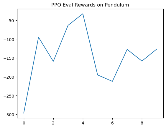
from stable_baselines3 import PPO
from stable_baselines3.common.env_util import make_vec_env
from stable_baselines3.common.evaluation import evaluate_policy
import gymnasium as gym
import numpy as np
import matplotlib.pyplot as plt
from matplotlib import animation
from IPython.display import HTML

# Hyperparameters (tuned for better performance)
env_id = "Pendulum-v1"
num_envs = 4
vec_env = make_vec_env(env_id, n_envs=num_envs)

model = PPO("MlpPolicy", vec_env, verbose=1, n_steps=2048, batch_size=128, n_epochs=20, learning_rate=1e-3, clip_range=0.2)

# Training
model.learn(total_timesteps=500000)  # Increased

# Evaluation
mean_reward, std_reward = evaluate_policy(model, vec_env, n_eval_episodes=10)
print(f"Mean Reward: {mean_reward:.2f} +/- {std_reward:.2f}")

# Animation for one episode using a single env
single_env = gym.make(env_id, render_mode='rgb_array')
obs, _ = single_env.reset()
frames = []
done = False
step = 0
max_steps = 300  # Limit for visualization
while not done and step < max_steps:
    frame = single_env.render()
    frames.append(frame)
    action, _ = model.predict(obs, deterministic=True)
    obs, _, done, _, _ = single_env.step(action)
    step += 1
single_env.close()

# Display animation
fig = plt.figure(figsize=(6, 6))
img = plt.imshow(frames[0])
plt.axis('off')
def animate(i):
    img.set_array(frames[i])
    return [img]
anim = animation.FuncAnimation(fig, animate, frames=len(frames), interval=50, blit=True)
plt.close(fig)
HTML(anim.to_jshtml())

Using cuda device
----------------------------------
| rollout/           |           |
|    ep_len_mean     | 200       |
|    ep_rew_mean     | -1.24e+03 |
| time/              |           |
|    fps             | 8852      |
|    iterations      | 1         |
|    time_elapsed    | 0         |
|    total_timesteps | 8192      |
----------------------------------
------------------------------------------
| rollout/                |              |
|    ep_len_mean          | 200          |
|    ep_rew_mean          | -1.18e+03    |
| time/                   |              |
|    fps                  | 4283         |
|    iterations           | 2            |
|    time_elapsed         | 3            |
|    total_timesteps      | 16384        |
| train/                  |              |
|    approx_kl            | 0.0040132715 |
|    clip_fraction        | 0.035        |
|    clip_range           | 0.2          |
|    entropy_loss         | -1.4         |
|    explained_variance   | -0.0027      |
|    learning_rate        | 0.001        |
|    loss                 | 445          |
|    n_updates            | 20           |
|    policy_gradient_loss | -0.00145     |
|    std                  | 0.978        |
|    value_loss           | 3.82e+03     |
------------------------------------------
-----------------------------------------
| rollout/                |             |
|    ep_len_mean          | 200         |
|    ep_rew_mean          | -1.17e+03   |
| time/                   |             |
|    fps                  | 3665        |
|    iterations           | 3           |
|    time_elapsed         | 6           |
|    total_timesteps      | 24576       |
| train/                  |             |
|    approx_kl            | 0.003162979 |
|    clip_fraction        | 0.0228      |
|    clip_range           | 0.2         |
|    entropy_loss         | -1.4        |
|    explained_variance   | 0.483       |
|    learning_rate        | 0.001       |
|    loss                 | 301         |
|    n_updates            | 40          |
|    policy_gradient_loss | -0.00119    |
|    std                  | 0.979       |
|    value_loss           | 1.97e+03    |
-----------------------------------------
-----------------------------------------
| rollout/                |             |
|    ep_len_mean          | 200         |
|    ep_rew_mean          | -1.15e+03   |
| time/                   |             |
|    fps                  | 3426        |
|    iterations           | 4           |
|    time_elapsed         | 9           |
|    total_timesteps      | 32768       |
| train/                  |             |
|    approx_kl            | 0.004853309 |
|    clip_fraction        | 0.046       |
|    clip_range           | 0.2         |
|    entropy_loss         | -1.38       |
|    explained_variance   | 0.589       |
|    learning_rate        | 0.001       |
|    loss                 | 205         |
|    n_updates            | 60          |
|    policy_gradient_loss | -0.0025     |
|    std                  | 0.958       |
|    value_loss           | 1.4e+03     |
-----------------------------------------
-----------------------------------------
| rollout/                |             |
|    ep_len_mean          | 200         |
|    ep_rew_mean          | -1.09e+03   |
| time/                   |             |
|    fps                  | 3298        |
|    iterations           | 5           |
|    time_elapsed         | 12          |
|    total_timesteps      | 40960       |
| train/                  |             |
|    approx_kl            | 0.004547151 |
|    clip_fraction        | 0.0419      |
|    clip_range           | 0.2         |
|    entropy_loss         | -1.37       |
|    explained_variance   | 0.73        |
|    learning_rate        | 0.001       |
|    loss                 | 188         |
|    n_updates            | 80          |
|    policy_gradient_loss | -0.00311    |
|    std                  | 0.953       |
|    value_loss           | 1.08e+03    |
-----------------------------------------
-----------------------------------------
| rollout/                |             |
|    ep_len_mean          | 200         |
|    ep_rew_mean          | -1.08e+03   |
| time/                   |             |
|    fps                  | 3217        |
|    iterations           | 6           |
|    time_elapsed         | 15          |
|    total_timesteps      | 49152       |
| train/                  |             |
|    approx_kl            | 0.006411713 |
|    clip_fraction        | 0.0559      |
|    clip_range           | 0.2         |
|    entropy_loss         | -1.36       |
|    explained_variance   | 0.817       |
|    learning_rate        | 0.001       |
|    loss                 | 144         |
|    n_updates            | 100         |
|    policy_gradient_loss | -0.00433    |
|    std                  | 0.947       |
|    value_loss           | 563         |
-----------------------------------------
-----------------------------------------
| rollout/                |             |
|    ep_len_mean          | 200         |
|    ep_rew_mean          | -1.03e+03   |
| time/                   |             |
|    fps                  | 3162        |
|    iterations           | 7           |
|    time_elapsed         | 18          |
|    total_timesteps      | 57344       |
| train/                  |             |
|    approx_kl            | 0.007908376 |
|    clip_fraction        | 0.0854      |
|    clip_range           | 0.2         |
|    entropy_loss         | -1.35       |
|    explained_variance   | 0.846       |
|    learning_rate        | 0.001       |
|    loss                 | 77.3        |
|    n_updates            | 120         |
|    policy_gradient_loss | -0.00516    |
|    std                  | 0.923       |
|    value_loss           | 456         |
-----------------------------------------
-----------------------------------------
| rollout/                |             |
|    ep_len_mean          | 200         |
|    ep_rew_mean          | -971        |
| time/                   |             |
|    fps                  | 3120        |
|    iterations           | 8           |
|    time_elapsed         | 21          |
|    total_timesteps      | 65536       |
| train/                  |             |
|    approx_kl            | 0.009165777 |
|    clip_fraction        | 0.104       |
|    clip_range           | 0.2         |
|    entropy_loss         | -1.33       |
|    explained_variance   | 0.891       |
|    learning_rate        | 0.001       |
|    loss                 | 118         |
|    n_updates            | 140         |
|    policy_gradient_loss | -0.00733    |
|    std                  | 0.923       |
|    value_loss           | 331         |
-----------------------------------------
----------------------------------------
| rollout/                |            |
|    ep_len_mean          | 200        |
|    ep_rew_mean          | -916       |
| time/                   |            |
|    fps                  | 3087       |
|    iterations           | 9          |
|    time_elapsed         | 23         |
|    total_timesteps      | 73728      |
| train/                  |            |
|    approx_kl            | 0.01744076 |
|    clip_fraction        | 0.161      |
|    clip_range           | 0.2        |
|    entropy_loss         | -1.32      |
|    explained_variance   | 0.894      |
|    learning_rate        | 0.001      |
|    loss                 | 87.8       |
|    n_updates            | 160        |
|    policy_gradient_loss | -0.0134    |
|    std                  | 0.906      |
|    value_loss           | 212        |
----------------------------------------
-----------------------------------------
| rollout/                |             |
|    ep_len_mean          | 200         |
|    ep_rew_mean          | -845        |
| time/                   |             |
|    fps                  | 3062        |
|    iterations           | 10          |
|    time_elapsed         | 26          |
|    total_timesteps      | 81920       |
| train/                  |             |
|    approx_kl            | 0.013182394 |
|    clip_fraction        | 0.168       |
|    clip_range           | 0.2         |
|    entropy_loss         | -1.3        |
|    explained_variance   | 0.889       |
|    learning_rate        | 0.001       |
|    loss                 | 82.2        |
|    n_updates            | 180         |
|    policy_gradient_loss | -0.0134     |
|    std                  | 0.882       |
|    value_loss           | 189         |
-----------------------------------------
-----------------------------------------
| rollout/                |             |
|    ep_len_mean          | 200         |
|    ep_rew_mean          | -732        |
| time/                   |             |
|    fps                  | 3043        |
|    iterations           | 11          |
|    time_elapsed         | 29          |
|    total_timesteps      | 90112       |
| train/                  |             |
|    approx_kl            | 0.020248545 |
|    clip_fraction        | 0.202       |
|    clip_range           | 0.2         |
|    entropy_loss         | -1.26       |
|    explained_variance   | 0.896       |
|    learning_rate        | 0.001       |
|    loss                 | 81.7        |
|    n_updates            | 200         |
|    policy_gradient_loss | -0.0183     |
|    std                  | 0.848       |
|    value_loss           | 211         |
-----------------------------------------
-----------------------------------------
| rollout/                |             |
|    ep_len_mean          | 200         |
|    ep_rew_mean          | -552        |
| time/                   |             |
|    fps                  | 3027        |
|    iterations           | 12          |
|    time_elapsed         | 32          |
|    total_timesteps      | 98304       |
| train/                  |             |
|    approx_kl            | 0.018160578 |
|    clip_fraction        | 0.201       |
|    clip_range           | 0.2         |
|    entropy_loss         | -1.22       |
|    explained_variance   | 0.841       |
|    learning_rate        | 0.001       |
|    loss                 | 138         |
|    n_updates            | 220         |
|    policy_gradient_loss | -0.0216     |
|    std                  | 0.819       |
|    value_loss           | 292         |
-----------------------------------------
---------------------------------------
| rollout/                |           |
|    ep_len_mean          | 200       |
|    ep_rew_mean          | -404      |
| time/                   |           |
|    fps                  | 3014      |
|    iterations           | 13        |
|    time_elapsed         | 35        |
|    total_timesteps      | 106496    |
| train/                  |           |
|    approx_kl            | 0.0144472 |
|    clip_fraction        | 0.176     |
|    clip_range           | 0.2       |
|    entropy_loss         | -1.18     |
|    explained_variance   | 0.888     |
|    learning_rate        | 0.001     |
|    loss                 | 143       |
|    n_updates            | 240       |
|    policy_gradient_loss | -0.019    |
|    std                  | 0.784     |
|    value_loss           | 305       |
---------------------------------------
-----------------------------------------
| rollout/                |             |
|    ep_len_mean          | 200         |
|    ep_rew_mean          | -313        |
| time/                   |             |
|    fps                  | 3002        |
|    iterations           | 14          |
|    time_elapsed         | 38          |
|    total_timesteps      | 114688      |
| train/                  |             |
|    approx_kl            | 0.012454664 |
|    clip_fraction        | 0.16        |
|    clip_range           | 0.2         |
|    entropy_loss         | -1.14       |
|    explained_variance   | 0.94        |
|    learning_rate        | 0.001       |
|    loss                 | 86.6        |
|    n_updates            | 260         |
|    policy_gradient_loss | -0.0115     |
|    std                  | 0.759       |
|    value_loss           | 187         |
-----------------------------------------
------------------------------------------
| rollout/                |              |
|    ep_len_mean          | 200          |
|    ep_rew_mean          | -239         |
| time/                   |              |
|    fps                  | 2991         |
|    iterations           | 15           |
|    time_elapsed         | 41           |
|    total_timesteps      | 122880       |
| train/                  |              |
|    approx_kl            | 0.0135291945 |
|    clip_fraction        | 0.132        |
|    clip_range           | 0.2          |
|    entropy_loss         | -1.11        |
|    explained_variance   | 0.97         |
|    learning_rate        | 0.001        |
|    loss                 | 30.6         |
|    n_updates            | 280          |
|    policy_gradient_loss | -0.00384     |
|    std                  | 0.73         |
|    value_loss           | 80.3         |
------------------------------------------
-----------------------------------------
| rollout/                |             |
|    ep_len_mean          | 200         |
|    ep_rew_mean          | -208        |
| time/                   |             |
|    fps                  | 2982        |
|    iterations           | 16          |
|    time_elapsed         | 43          |
|    total_timesteps      | 131072      |
| train/                  |             |
|    approx_kl            | 0.007148423 |
|    clip_fraction        | 0.125       |
|    clip_range           | 0.2         |
|    entropy_loss         | -1.1        |
|    explained_variance   | 0.973       |
|    learning_rate        | 0.001       |
|    loss                 | 26.8        |
|    n_updates            | 300         |
|    policy_gradient_loss | 0.00108     |
|    std                  | 0.729       |
|    value_loss           | 49.9        |
-----------------------------------------
------------------------------------------
| rollout/                |              |
|    ep_len_mean          | 200          |
|    ep_rew_mean          | -206         |
| time/                   |              |
|    fps                  | 2974         |
|    iterations           | 17           |
|    time_elapsed         | 46           |
|    total_timesteps      | 139264       |
| train/                  |              |
|    approx_kl            | 0.0087289065 |
|    clip_fraction        | 0.111        |
|    clip_range           | 0.2          |
|    entropy_loss         | -1.09        |
|    explained_variance   | 0.975        |
|    learning_rate        | 0.001        |
|    loss                 | 15.4         |
|    n_updates            | 320          |
|    policy_gradient_loss | 0.00115      |
|    std                  | 0.712        |
|    value_loss           | 46.5         |
------------------------------------------
-----------------------------------------
| rollout/                |             |
|    ep_len_mean          | 200         |
|    ep_rew_mean          | -198        |
| time/                   |             |
|    fps                  | 2967        |
|    iterations           | 18          |
|    time_elapsed         | 49          |
|    total_timesteps      | 147456      |
| train/                  |             |
|    approx_kl            | 0.015821712 |
|    clip_fraction        | 0.115       |
|    clip_range           | 0.2         |
|    entropy_loss         | -1.04       |
|    explained_variance   | 0.958       |
|    learning_rate        | 0.001       |
|    loss                 | 55.2        |
|    n_updates            | 340         |
|    policy_gradient_loss | -0.00648    |
|    std                  | 0.678       |
|    value_loss           | 90.8        |
-----------------------------------------
------------------------------------------
| rollout/                |              |
|    ep_len_mean          | 200          |
|    ep_rew_mean          | -194         |
| time/                   |              |
|    fps                  | 2962         |
|    iterations           | 19           |
|    time_elapsed         | 52           |
|    total_timesteps      | 155648       |
| train/                  |              |
|    approx_kl            | 0.0062003215 |
|    clip_fraction        | 0.135        |
|    clip_range           | 0.2          |
|    entropy_loss         | -1.01        |
|    explained_variance   | 0.977        |
|    learning_rate        | 0.001        |
|    loss                 | 28.3         |
|    n_updates            | 360          |
|    policy_gradient_loss | 0.00339      |
|    std                  | 0.661        |
|    value_loss           | 32.9         |
------------------------------------------
------------------------------------------
| rollout/                |              |
|    ep_len_mean          | 200          |
|    ep_rew_mean          | -171         |
| time/                   |              |
|    fps                  | 2957         |
|    iterations           | 20           |
|    time_elapsed         | 55           |
|    total_timesteps      | 163840       |
| train/                  |              |
|    approx_kl            | 0.0072847046 |
|    clip_fraction        | 0.119        |
|    clip_range           | 0.2          |
|    entropy_loss         | -0.996       |
|    explained_variance   | 0.985        |
|    learning_rate        | 0.001        |
|    loss                 | 4.88         |
|    n_updates            | 380          |
|    policy_gradient_loss | 0.00364      |
|    std                  | 0.654        |
|    value_loss           | 18.3         |
------------------------------------------
-----------------------------------------
| rollout/                |             |
|    ep_len_mean          | 200         |
|    ep_rew_mean          | -176        |
| time/                   |             |
|    fps                  | 2952        |
|    iterations           | 21          |
|    time_elapsed         | 58          |
|    total_timesteps      | 172032      |
| train/                  |             |
|    approx_kl            | 0.006490346 |
|    clip_fraction        | 0.112       |
|    clip_range           | 0.2         |
|    entropy_loss         | -0.978      |
|    explained_variance   | 0.987       |
|    learning_rate        | 0.001       |
|    loss                 | 2.96        |
|    n_updates            | 400         |
|    policy_gradient_loss | 0.00394     |
|    std                  | 0.644       |
|    value_loss           | 13.3        |
-----------------------------------------
-----------------------------------------
| rollout/                |             |
|    ep_len_mean          | 200         |
|    ep_rew_mean          | -179        |
| time/                   |             |
|    fps                  | 2948        |
|    iterations           | 22          |
|    time_elapsed         | 61          |
|    total_timesteps      | 180224      |
| train/                  |             |
|    approx_kl            | 0.009609673 |
|    clip_fraction        | 0.0816      |
|    clip_range           | 0.2         |
|    entropy_loss         | -0.953      |
|    explained_variance   | 0.982       |
|    learning_rate        | 0.001       |
|    loss                 | 21.5        |
|    n_updates            | 420         |
|    policy_gradient_loss | -0.000956   |
|    std                  | 0.62        |
|    value_loss           | 27.7        |
-----------------------------------------
-----------------------------------------
| rollout/                |             |
|    ep_len_mean          | 200         |
|    ep_rew_mean          | -175        |
| time/                   |             |
|    fps                  | 2944        |
|    iterations           | 23          |
|    time_elapsed         | 63          |
|    total_timesteps      | 188416      |
| train/                  |             |
|    approx_kl            | 0.010505131 |
|    clip_fraction        | 0.0966      |
|    clip_range           | 0.2         |
|    entropy_loss         | -0.936      |
|    explained_variance   | 0.981       |
|    learning_rate        | 0.001       |
|    loss                 | 10.5        |
|    n_updates            | 440         |
|    policy_gradient_loss | 0.00112     |
|    std                  | 0.623       |
|    value_loss           | 26.4        |
-----------------------------------------
-----------------------------------------
| rollout/                |             |
|    ep_len_mean          | 200         |
|    ep_rew_mean          | -170        |
| time/                   |             |
|    fps                  | 2941        |
|    iterations           | 24          |
|    time_elapsed         | 66          |
|    total_timesteps      | 196608      |
| train/                  |             |
|    approx_kl            | 0.009774239 |
|    clip_fraction        | 0.132       |
|    clip_range           | 0.2         |
|    entropy_loss         | -0.917      |
|    explained_variance   | 0.985       |
|    learning_rate        | 0.001       |
|    loss                 | 2.52        |
|    n_updates            | 460         |
|    policy_gradient_loss | 0.00324     |
|    std                  | 0.604       |
|    value_loss           | 10.3        |
-----------------------------------------
-----------------------------------------
| rollout/                |             |
|    ep_len_mean          | 200         |
|    ep_rew_mean          | -168        |
| time/                   |             |
|    fps                  | 2938        |
|    iterations           | 25          |
|    time_elapsed         | 69          |
|    total_timesteps      | 204800      |
| train/                  |             |
|    approx_kl            | 0.011115698 |
|    clip_fraction        | 0.115       |
|    clip_range           | 0.2         |
|    entropy_loss         | -0.879      |
|    explained_variance   | 0.985       |
|    learning_rate        | 0.001       |
|    loss                 | 4.07        |
|    n_updates            | 480         |
|    policy_gradient_loss | 0.000982    |
|    std                  | 0.578       |
|    value_loss           | 13.5        |
-----------------------------------------
-----------------------------------------
| rollout/                |             |
|    ep_len_mean          | 200         |
|    ep_rew_mean          | -159        |
| time/                   |             |
|    fps                  | 2935        |
|    iterations           | 26          |
|    time_elapsed         | 72          |
|    total_timesteps      | 212992      |
| train/                  |             |
|    approx_kl            | 0.021236617 |
|    clip_fraction        | 0.123       |
|    clip_range           | 0.2         |
|    entropy_loss         | -0.874      |
|    explained_variance   | 0.985       |
|    learning_rate        | 0.001       |
|    loss                 | 1.2         |
|    n_updates            | 500         |
|    policy_gradient_loss | 0.00345     |
|    std                  | 0.582       |
|    value_loss           | 6.26        |
-----------------------------------------
-----------------------------------------
| rollout/                |             |
|    ep_len_mean          | 200         |
|    ep_rew_mean          | -159        |
| time/                   |             |
|    fps                  | 2932        |
|    iterations           | 27          |
|    time_elapsed         | 75          |
|    total_timesteps      | 221184      |
| train/                  |             |
|    approx_kl            | 0.012304497 |
|    clip_fraction        | 0.135       |
|    clip_range           | 0.2         |
|    entropy_loss         | -0.877      |
|    explained_variance   | 0.984       |
|    learning_rate        | 0.001       |
|    loss                 | 1.25        |
|    n_updates            | 520         |
|    policy_gradient_loss | 0.0033      |
|    std                  | 0.585       |
|    value_loss           | 9.64        |
-----------------------------------------
-----------------------------------------
| rollout/                |             |
|    ep_len_mean          | 200         |
|    ep_rew_mean          | -169        |
| time/                   |             |
|    fps                  | 2929        |
|    iterations           | 28          |
|    time_elapsed         | 78          |
|    total_timesteps      | 229376      |
| train/                  |             |
|    approx_kl            | 0.012314701 |
|    clip_fraction        | 0.0884      |
|    clip_range           | 0.2         |
|    entropy_loss         | -0.877      |
|    explained_variance   | 0.991       |
|    learning_rate        | 0.001       |
|    loss                 | 3.55        |
|    n_updates            | 540         |
|    policy_gradient_loss | -0.000728   |
|    std                  | 0.584       |
|    value_loss           | 9.11        |
-----------------------------------------
------------------------------------------
| rollout/                |              |
|    ep_len_mean          | 200          |
|    ep_rew_mean          | -187         |
| time/                   |              |
|    fps                  | 2925         |
|    iterations           | 29           |
|    time_elapsed         | 81           |
|    total_timesteps      | 237568       |
| train/                  |              |
|    approx_kl            | 0.0089102555 |
|    clip_fraction        | 0.0669       |
|    clip_range           | 0.2          |
|    entropy_loss         | -0.877       |
|    explained_variance   | 0.955        |
|    learning_rate        | 0.001        |
|    loss                 | 14           |
|    n_updates            | 560          |
|    policy_gradient_loss | -0.00258     |
|    std                  | 0.58         |
|    value_loss           | 45.9         |
------------------------------------------
------------------------------------------
| rollout/                |              |
|    ep_len_mean          | 200          |
|    ep_rew_mean          | -175         |
| time/                   |              |
|    fps                  | 2923         |
|    iterations           | 30           |
|    time_elapsed         | 84           |
|    total_timesteps      | 245760       |
| train/                  |              |
|    approx_kl            | 0.0036787807 |
|    clip_fraction        | 0.0422       |
|    clip_range           | 0.2          |
|    entropy_loss         | -0.885       |
|    explained_variance   | 0.91         |
|    learning_rate        | 0.001        |
|    loss                 | 74.9         |
|    n_updates            | 580          |
|    policy_gradient_loss | -0.0062      |
|    std                  | 0.595        |
|    value_loss           | 127          |
------------------------------------------
-----------------------------------------
| rollout/                |             |
|    ep_len_mean          | 200         |
|    ep_rew_mean          | -170        |
| time/                   |             |
|    fps                  | 2921        |
|    iterations           | 31          |
|    time_elapsed         | 86          |
|    total_timesteps      | 253952      |
| train/                  |             |
|    approx_kl            | 0.020262873 |
|    clip_fraction        | 0.148       |
|    clip_range           | 0.2         |
|    entropy_loss         | -0.899      |
|    explained_variance   | 0.97        |
|    learning_rate        | 0.001       |
|    loss                 | 2.59        |
|    n_updates            | 600         |
|    policy_gradient_loss | 0.00625     |
|    std                  | 0.587       |
|    value_loss           | 18.9        |
-----------------------------------------
-----------------------------------------
| rollout/                |             |
|    ep_len_mean          | 200         |
|    ep_rew_mean          | -175        |
| time/                   |             |
|    fps                  | 2919        |
|    iterations           | 32          |
|    time_elapsed         | 89          |
|    total_timesteps      | 262144      |
| train/                  |             |
|    approx_kl            | 0.015241284 |
|    clip_fraction        | 0.115       |
|    clip_range           | 0.2         |
|    entropy_loss         | -0.855      |
|    explained_variance   | 0.982       |
|    learning_rate        | 0.001       |
|    loss                 | 7.08        |
|    n_updates            | 620         |
|    policy_gradient_loss | 2.14e-05    |
|    std                  | 0.563       |
|    value_loss           | 10.8        |
-----------------------------------------
------------------------------------------
| rollout/                |              |
|    ep_len_mean          | 200          |
|    ep_rew_mean          | -169         |
| time/                   |              |
|    fps                  | 2918         |
|    iterations           | 33           |
|    time_elapsed         | 92           |
|    total_timesteps      | 270336       |
| train/                  |              |
|    approx_kl            | 0.0055862134 |
|    clip_fraction        | 0.0478       |
|    clip_range           | 0.2          |
|    entropy_loss         | -0.84        |
|    explained_variance   | 0.946        |
|    learning_rate        | 0.001        |
|    loss                 | 34.2         |
|    n_updates            | 640          |
|    policy_gradient_loss | -0.00398     |
|    std                  | 0.556        |
|    value_loss           | 49.4         |
------------------------------------------
-----------------------------------------
| rollout/                |             |
|    ep_len_mean          | 200         |
|    ep_rew_mean          | -158        |
| time/                   |             |
|    fps                  | 2916        |
|    iterations           | 34          |
|    time_elapsed         | 95          |
|    total_timesteps      | 278528      |
| train/                  |             |
|    approx_kl            | 0.010519964 |
|    clip_fraction        | 0.126       |
|    clip_range           | 0.2         |
|    entropy_loss         | -0.823      |
|    explained_variance   | 0.991       |
|    learning_rate        | 0.001       |
|    loss                 | 0.724       |
|    n_updates            | 660         |
|    policy_gradient_loss | 0.00908     |
|    std                  | 0.545       |
|    value_loss           | 1.79        |
-----------------------------------------
-----------------------------------------
| rollout/                |             |
|    ep_len_mean          | 200         |
|    ep_rew_mean          | -161        |
| time/                   |             |
|    fps                  | 2915        |
|    iterations           | 35          |
|    time_elapsed         | 98          |
|    total_timesteps      | 286720      |
| train/                  |             |
|    approx_kl            | 0.009506008 |
|    clip_fraction        | 0.0845      |
|    clip_range           | 0.2         |
|    entropy_loss         | -0.822      |
|    explained_variance   | 0.989       |
|    learning_rate        | 0.001       |
|    loss                 | 19          |
|    n_updates            | 680         |
|    policy_gradient_loss | 0.00156     |
|    std                  | 0.55        |
|    value_loss           | 12.5        |
-----------------------------------------
-----------------------------------------
| rollout/                |             |
|    ep_len_mean          | 200         |
|    ep_rew_mean          | -159        |
| time/                   |             |
|    fps                  | 2913        |
|    iterations           | 36          |
|    time_elapsed         | 101         |
|    total_timesteps      | 294912      |
| train/                  |             |
|    approx_kl            | 0.013374235 |
|    clip_fraction        | 0.0692      |
|    clip_range           | 0.2         |
|    entropy_loss         | -0.849      |
|    explained_variance   | 0.984       |
|    learning_rate        | 0.001       |
|    loss                 | 10.1        |
|    n_updates            | 700         |
|    policy_gradient_loss | -0.000656   |
|    std                  | 0.572       |
|    value_loss           | 16.6        |
-----------------------------------------
-----------------------------------------
| rollout/                |             |
|    ep_len_mean          | 200         |
|    ep_rew_mean          | -150        |
| time/                   |             |
|    fps                  | 2912        |
|    iterations           | 37          |
|    time_elapsed         | 104         |
|    total_timesteps      | 303104      |
| train/                  |             |
|    approx_kl            | 0.013946901 |
|    clip_fraction        | 0.128       |
|    clip_range           | 0.2         |
|    entropy_loss         | -0.857      |
|    explained_variance   | 0.99        |
|    learning_rate        | 0.001       |
|    loss                 | 1.01        |
|    n_updates            | 720         |
|    policy_gradient_loss | 0.00285     |
|    std                  | 0.558       |
|    value_loss           | 1.46        |
-----------------------------------------
-----------------------------------------
| rollout/                |             |
|    ep_len_mean          | 200         |
|    ep_rew_mean          | -144        |
| time/                   |             |
|    fps                  | 2910        |
|    iterations           | 38          |
|    time_elapsed         | 106         |
|    total_timesteps      | 311296      |
| train/                  |             |
|    approx_kl            | 0.014579998 |
|    clip_fraction        | 0.127       |
|    clip_range           | 0.2         |
|    entropy_loss         | -0.801      |
|    explained_variance   | 0.993       |
|    learning_rate        | 0.001       |
|    loss                 | 0.386       |
|    n_updates            | 740         |
|    policy_gradient_loss | 0.00375     |
|    std                  | 0.53        |
|    value_loss           | 0.727       |
-----------------------------------------
----------------------------------------
| rollout/                |            |
|    ep_len_mean          | 200        |
|    ep_rew_mean          | -154       |
| time/                   |            |
|    fps                  | 2909       |
|    iterations           | 39         |
|    time_elapsed         | 109        |
|    total_timesteps      | 319488     |
| train/                  |            |
|    approx_kl            | 0.01269204 |
|    clip_fraction        | 0.118      |
|    clip_range           | 0.2        |
|    entropy_loss         | -0.763     |
|    explained_variance   | 0.999      |
|    learning_rate        | 0.001      |
|    loss                 | 0.247      |
|    n_updates            | 760        |
|    policy_gradient_loss | 0.00355    |
|    std                  | 0.512      |
|    value_loss           | 0.707      |
----------------------------------------
-----------------------------------------
| rollout/                |             |
|    ep_len_mean          | 200         |
|    ep_rew_mean          | -158        |
| time/                   |             |
|    fps                  | 2908        |
|    iterations           | 40          |
|    time_elapsed         | 112         |
|    total_timesteps      | 327680      |
| train/                  |             |
|    approx_kl            | 0.010248585 |
|    clip_fraction        | 0.0989      |
|    clip_range           | 0.2         |
|    entropy_loss         | -0.743      |
|    explained_variance   | 0.996       |
|    learning_rate        | 0.001       |
|    loss                 | 0.249       |
|    n_updates            | 780         |
|    policy_gradient_loss | 0.000575    |
|    std                  | 0.504       |
|    value_loss           | 0.632       |
-----------------------------------------
-----------------------------------------
| rollout/                |             |
|    ep_len_mean          | 200         |
|    ep_rew_mean          | -154        |
| time/                   |             |
|    fps                  | 2907        |
|    iterations           | 41          |
|    time_elapsed         | 115         |
|    total_timesteps      | 335872      |
| train/                  |             |
|    approx_kl            | 0.011398923 |
|    clip_fraction        | 0.116       |
|    clip_range           | 0.2         |
|    entropy_loss         | -0.742      |
|    explained_variance   | 0.997       |
|    learning_rate        | 0.001       |
|    loss                 | 0.48        |
|    n_updates            | 800         |
|    policy_gradient_loss | -0.00174    |
|    std                  | 0.51        |
|    value_loss           | 1.8         |
-----------------------------------------
-----------------------------------------
| rollout/                |             |
|    ep_len_mean          | 200         |
|    ep_rew_mean          | -147        |
| time/                   |             |
|    fps                  | 2906        |
|    iterations           | 42          |
|    time_elapsed         | 118         |
|    total_timesteps      | 344064      |
| train/                  |             |
|    approx_kl            | 0.010751015 |
|    clip_fraction        | 0.159       |
|    clip_range           | 0.2         |
|    entropy_loss         | -0.744      |
|    explained_variance   | 0.994       |
|    learning_rate        | 0.001       |
|    loss                 | 0.0767      |
|    n_updates            | 820         |
|    policy_gradient_loss | 0.00411     |
|    std                  | 0.504       |
|    value_loss           | 1.21        |
-----------------------------------------
----------------------------------------
| rollout/                |            |
|    ep_len_mean          | 200        |
|    ep_rew_mean          | -155       |
| time/                   |            |
|    fps                  | 2905       |
|    iterations           | 43         |
|    time_elapsed         | 121        |
|    total_timesteps      | 352256     |
| train/                  |            |
|    approx_kl            | 0.02714363 |
|    clip_fraction        | 0.134      |
|    clip_range           | 0.2        |
|    entropy_loss         | -0.728     |
|    explained_variance   | 0.996      |
|    learning_rate        | 0.001      |
|    loss                 | 8.89       |
|    n_updates            | 840        |
|    policy_gradient_loss | 0.00335    |
|    std                  | 0.505      |
|    value_loss           | 1.69       |
----------------------------------------
-----------------------------------------
| rollout/                |             |
|    ep_len_mean          | 200         |
|    ep_rew_mean          | -151        |
| time/                   |             |
|    fps                  | 2904        |
|    iterations           | 44          |
|    time_elapsed         | 124         |
|    total_timesteps      | 360448      |
| train/                  |             |
|    approx_kl            | 0.007602521 |
|    clip_fraction        | 0.0853      |
|    clip_range           | 0.2         |
|    entropy_loss         | -0.722      |
|    explained_variance   | 0.976       |
|    learning_rate        | 0.001       |
|    loss                 | 0.379       |
|    n_updates            | 860         |
|    policy_gradient_loss | -0.000521   |
|    std                  | 0.492       |
|    value_loss           | 12.4        |
-----------------------------------------
----------------------------------------
| rollout/                |            |
|    ep_len_mean          | 200        |
|    ep_rew_mean          | -161       |
| time/                   |            |
|    fps                  | 2903       |
|    iterations           | 45         |
|    time_elapsed         | 126        |
|    total_timesteps      | 368640     |
| train/                  |            |
|    approx_kl            | 0.14335462 |
|    clip_fraction        | 0.162      |
|    clip_range           | 0.2        |
|    entropy_loss         | -0.739     |
|    explained_variance   | 0.998      |
|    learning_rate        | 0.001      |
|    loss                 | 0.0359     |
|    n_updates            | 880        |
|    policy_gradient_loss | 0.0159     |
|    std                  | 0.496      |
|    value_loss           | 0.311      |
----------------------------------------
-----------------------------------------
| rollout/                |             |
|    ep_len_mean          | 200         |
|    ep_rew_mean          | -195        |
| time/                   |             |
|    fps                  | 2902        |
|    iterations           | 46          |
|    time_elapsed         | 129         |
|    total_timesteps      | 376832      |
| train/                  |             |
|    approx_kl            | 0.012488343 |
|    clip_fraction        | 0.0605      |
|    clip_range           | 0.2         |
|    entropy_loss         | -0.739      |
|    explained_variance   | 0.948       |
|    learning_rate        | 0.001       |
|    loss                 | 3.76        |
|    n_updates            | 900         |
|    policy_gradient_loss | 0.00358     |
|    std                  | 0.518       |
|    value_loss           | 8.08        |
-----------------------------------------
-----------------------------------------
| rollout/                |             |
|    ep_len_mean          | 200         |
|    ep_rew_mean          | -196        |
| time/                   |             |
|    fps                  | 2902        |
|    iterations           | 47          |
|    time_elapsed         | 132         |
|    total_timesteps      | 385024      |
| train/                  |             |
|    approx_kl            | 0.009624409 |
|    clip_fraction        | 0.0669      |
|    clip_range           | 0.2         |
|    entropy_loss         | -0.784      |
|    explained_variance   | 0.988       |
|    learning_rate        | 0.001       |
|    loss                 | 2.71        |
|    n_updates            | 920         |
|    policy_gradient_loss | -0.00446    |
|    std                  | 0.527       |
|    value_loss           | 10.7        |
-----------------------------------------
-----------------------------------------
| rollout/                |             |
|    ep_len_mean          | 200         |
|    ep_rew_mean          | -191        |
| time/                   |             |
|    fps                  | 2901        |
|    iterations           | 48          |
|    time_elapsed         | 135         |
|    total_timesteps      | 393216      |
| train/                  |             |
|    approx_kl            | 0.010654209 |
|    clip_fraction        | 0.0926      |
|    clip_range           | 0.2         |
|    entropy_loss         | -0.816      |
|    explained_variance   | 0.995       |
|    learning_rate        | 0.001       |
|    loss                 | 0.467       |
|    n_updates            | 940         |
|    policy_gradient_loss | 0.00123     |
|    std                  | 0.563       |
|    value_loss           | 3.94        |
-----------------------------------------
-----------------------------------------
| rollout/                |             |
|    ep_len_mean          | 200         |
|    ep_rew_mean          | -182        |
| time/                   |             |
|    fps                  | 2900        |
|    iterations           | 49          |
|    time_elapsed         | 138         |
|    total_timesteps      | 401408      |
| train/                  |             |
|    approx_kl            | 0.013650073 |
|    clip_fraction        | 0.105       |
|    clip_range           | 0.2         |
|    entropy_loss         | -0.833      |
|    explained_variance   | 0.991       |
|    learning_rate        | 0.001       |
|    loss                 | 0.446       |
|    n_updates            | 960         |
|    policy_gradient_loss | 0.000896    |
|    std                  | 0.55        |
|    value_loss           | 8.22        |
-----------------------------------------
-----------------------------------------
| rollout/                |             |
|    ep_len_mean          | 200         |
|    ep_rew_mean          | -181        |
| time/                   |             |
|    fps                  | 2899        |
|    iterations           | 50          |
|    time_elapsed         | 141         |
|    total_timesteps      | 409600      |
| train/                  |             |
|    approx_kl            | 0.014310302 |
|    clip_fraction        | 0.164       |
|    clip_range           | 0.2         |
|    entropy_loss         | -0.778      |
|    explained_variance   | 0.994       |
|    learning_rate        | 0.001       |
|    loss                 | 2.93        |
|    n_updates            | 980         |
|    policy_gradient_loss | 0.00229     |
|    std                  | 0.534       |
|    value_loss           | 1.98        |
-----------------------------------------
---------------------------------------
| rollout/                |           |
|    ep_len_mean          | 200       |
|    ep_rew_mean          | -181      |
| time/                   |           |
|    fps                  | 2898      |
|    iterations           | 51        |
|    time_elapsed         | 144       |
|    total_timesteps      | 417792    |
| train/                  |           |
|    approx_kl            | 0.0314454 |
|    clip_fraction        | 0.184     |
|    clip_range           | 0.2       |
|    entropy_loss         | -0.758    |
|    explained_variance   | 0.994     |
|    learning_rate        | 0.001     |
|    loss                 | 0.341     |
|    n_updates            | 1000      |
|    policy_gradient_loss | 0.00172   |
|    std                  | 0.51      |
|    value_loss           | 1.53      |
---------------------------------------
-----------------------------------------
| rollout/                |             |
|    ep_len_mean          | 200         |
|    ep_rew_mean          | -178        |
| time/                   |             |
|    fps                  | 2897        |
|    iterations           | 52          |
|    time_elapsed         | 146         |
|    total_timesteps      | 425984      |
| train/                  |             |
|    approx_kl            | 0.011495896 |
|    clip_fraction        | 0.122       |
|    clip_range           | 0.2         |
|    entropy_loss         | -0.726      |
|    explained_variance   | 0.995       |
|    learning_rate        | 0.001       |
|    loss                 | 1.49        |
|    n_updates            | 1020        |
|    policy_gradient_loss | -0.00198    |
|    std                  | 0.495       |
|    value_loss           | 7.8         |
-----------------------------------------
-----------------------------------------
| rollout/                |             |
|    ep_len_mean          | 200         |
|    ep_rew_mean          | -168        |
| time/                   |             |
|    fps                  | 2897        |
|    iterations           | 53          |
|    time_elapsed         | 149         |
|    total_timesteps      | 434176      |
| train/                  |             |
|    approx_kl            | 0.016162075 |
|    clip_fraction        | 0.161       |
|    clip_range           | 0.2         |
|    entropy_loss         | -0.697      |
|    explained_variance   | 0.998       |
|    learning_rate        | 0.001       |
|    loss                 | 0.183       |
|    n_updates            | 1040        |
|    policy_gradient_loss | 0.00575     |
|    std                  | 0.478       |
|    value_loss           | 0.867       |
-----------------------------------------
-----------------------------------------
| rollout/                |             |
|    ep_len_mean          | 200         |
|    ep_rew_mean          | -174        |
| time/                   |             |
|    fps                  | 2896        |
|    iterations           | 54          |
|    time_elapsed         | 152         |
|    total_timesteps      | 442368      |
| train/                  |             |
|    approx_kl            | 0.023620857 |
|    clip_fraction        | 0.122       |
|    clip_range           | 0.2         |
|    entropy_loss         | -0.657      |
|    explained_variance   | 0.987       |
|    learning_rate        | 0.001       |
|    loss                 | 14.4        |
|    n_updates            | 1060        |
|    policy_gradient_loss | 0.00618     |
|    std                  | 0.456       |
|    value_loss           | 7.25        |
-----------------------------------------
------------------------------------------
| rollout/                |              |
|    ep_len_mean          | 200          |
|    ep_rew_mean          | -188         |
| time/                   |              |
|    fps                  | 2896         |
|    iterations           | 55           |
|    time_elapsed         | 155          |
|    total_timesteps      | 450560       |
| train/                  |              |
|    approx_kl            | 0.0029533012 |
|    clip_fraction        | 0.0342       |
|    clip_range           | 0.2          |
|    entropy_loss         | -0.642       |
|    explained_variance   | 0.898        |
|    learning_rate        | 0.001        |
|    loss                 | 8.88         |
|    n_updates            | 1080         |
|    policy_gradient_loss | -0.00261     |
|    std                  | 0.465        |
|    value_loss           | 51.5         |
------------------------------------------
------------------------------------------
| rollout/                |              |
|    ep_len_mean          | 200          |
|    ep_rew_mean          | -185         |
| time/                   |              |
|    fps                  | 2895         |
|    iterations           | 56           |
|    time_elapsed         | 158          |
|    total_timesteps      | 458752       |
| train/                  |              |
|    approx_kl            | 0.0026572794 |
|    clip_fraction        | 0.0241       |
|    clip_range           | 0.2          |
|    entropy_loss         | -0.651       |
|    explained_variance   | 0.956        |
|    learning_rate        | 0.001        |
|    loss                 | 60.9         |
|    n_updates            | 1100         |
|    policy_gradient_loss | -0.00544     |
|    std                  | 0.463        |
|    value_loss           | 94.7         |
------------------------------------------
-----------------------------------------
| rollout/                |             |
|    ep_len_mean          | 200         |
|    ep_rew_mean          | -172        |
| time/                   |             |
|    fps                  | 2894        |
|    iterations           | 57          |
|    time_elapsed         | 161         |
|    total_timesteps      | 466944      |
| train/                  |             |
|    approx_kl            | 0.009995181 |
|    clip_fraction        | 0.122       |
|    clip_range           | 0.2         |
|    entropy_loss         | -0.653      |
|    explained_variance   | 0.981       |
|    learning_rate        | 0.001       |
|    loss                 | 1.63        |
|    n_updates            | 1120        |
|    policy_gradient_loss | 0.00468     |
|    std                  | 0.465       |
|    value_loss           | 23.2        |
-----------------------------------------
-----------------------------------------
| rollout/                |             |
|    ep_len_mean          | 200         |
|    ep_rew_mean          | -197        |
| time/                   |             |
|    fps                  | 2894        |
|    iterations           | 58          |
|    time_elapsed         | 164         |
|    total_timesteps      | 475136      |
| train/                  |             |
|    approx_kl            | 0.023261528 |
|    clip_fraction        | 0.185       |
|    clip_range           | 0.2         |
|    entropy_loss         | -0.674      |
|    explained_variance   | 0.995       |
|    learning_rate        | 0.001       |
|    loss                 | 0.424       |
|    n_updates            | 1140        |
|    policy_gradient_loss | 0.00578     |
|    std                  | 0.478       |
|    value_loss           | 1.26        |
-----------------------------------------
------------------------------------------
| rollout/                |              |
|    ep_len_mean          | 200          |
|    ep_rew_mean          | -236         |
| time/                   |              |
|    fps                  | 2893         |
|    iterations           | 59           |
|    time_elapsed         | 167          |
|    total_timesteps      | 483328       |
| train/                  |              |
|    approx_kl            | 0.0060341065 |
|    clip_fraction        | 0.0455       |
|    clip_range           | 0.2          |
|    entropy_loss         | -0.702       |
|    explained_variance   | 0.879        |
|    learning_rate        | 0.001        |
|    loss                 | 17.5         |
|    n_updates            | 1160         |
|    policy_gradient_loss | -0.00283     |
|    std                  | 0.497        |
|    value_loss           | 43.6         |
------------------------------------------
------------------------------------------
| rollout/                |              |
|    ep_len_mean          | 200          |
|    ep_rew_mean          | -220         |
| time/                   |              |
|    fps                  | 2892         |
|    iterations           | 60           |
|    time_elapsed         | 169          |
|    total_timesteps      | 491520       |
| train/                  |              |
|    approx_kl            | 0.0044598775 |
|    clip_fraction        | 0.0411       |
|    clip_range           | 0.2          |
|    entropy_loss         | -0.737       |
|    explained_variance   | 0.939        |
|    learning_rate        | 0.001        |
|    loss                 | 93.3         |
|    n_updates            | 1180         |
|    policy_gradient_loss | -0.0065      |
|    std                  | 0.511        |
|    value_loss           | 114          |
------------------------------------------
-----------------------------------------
| rollout/                |             |
|    ep_len_mean          | 200         |
|    ep_rew_mean          | -202        |
| time/                   |             |
|    fps                  | 2891        |
|    iterations           | 61          |
|    time_elapsed         | 172         |
|    total_timesteps      | 499712      |
| train/                  |             |
|    approx_kl            | 0.046426184 |
|    clip_fraction        | 0.178       |
|    clip_range           | 0.2         |
|    entropy_loss         | -0.739      |
|    explained_variance   | 0.976       |
|    learning_rate        | 0.001       |
|    loss                 | 9.58        |
|    n_updates            | 1200        |
|    policy_gradient_loss | 0.00471     |
|    std                  | 0.504       |
|    value_loss           | 37          |
-----------------------------------------
-----------------------------------------
| rollout/                |             |
|    ep_len_mean          | 200         |
|    ep_rew_mean          | -181        |
| time/                   |             |
|    fps                  | 2890        |
|    iterations           | 62          |
|    time_elapsed         | 175         |
|    total_timesteps      | 507904      |
| train/                  |             |
|    approx_kl            | 0.015989544 |
|    clip_fraction        | 0.156       |
|    clip_range           | 0.2         |
|    entropy_loss         | -0.7        |
|    explained_variance   | 0.986       |
|    learning_rate        | 0.001       |
|    loss                 | 0.5         |
|    n_updates            | 1220        |
|    policy_gradient_loss | 0.00508     |
|    std                  | 0.483       |
|    value_loss           | 3.25        |
-----------------------------------------
Mean Reward: -160.35 +/- 109.37

Once Loop Reflect

This code learns to swing up and balance the pendulum, with rewards improving from ~ -1500 to ~ -100.

13.8.3 Actor-Critic Frameworks

Actor-critic methods separate the policy (actor) from value estimation (critic), using the critic to compute advantages for lower-variance gradients. Advantage Actor-Critic (A2C) synchronously collects data from multiple environments, updating the actor with \( \nabla_\theta \log \pi_\theta(a|s) \hat{A}(s,a) \) (where \( \hat{A} = Q(s,a) - V(s) \approx r + \gamma V(s') - V(s) \)) and the critic via TD errors. This balances bias-variance, enabling stable learning in continuous control.

A brief on Asynchronous A3C: Extends A2C with parallel actors on separate threads, asynchronously updating a shared model—improving exploration and speed, though with some staleness. In space applications, actor-critic suits hybrid discrete-continuous tasks like rover steering with energy constraints.

Example: A2C on MountainCar-v0

Below is a Python example of simple A2C (synchronous actor-critic) using PyTorch on Gymnasium’s MountainCar-v0 (discrete actions: left/none/right; continuous state: position/velocity; goal: reach flag). State relates to \( \mathbf{y} \), actions to discrete \( u \).

import gymnasium as gym
import numpy as np
import torch
import torch.nn as nn
import torch.optim as optim
import matplotlib.pyplot as plt
from IPython.display import HTML, display
from matplotlib import animation

# Hyperparameters
env = gym.make('MountainCar-v0')
state_dim = env.observation_space.shape[0]  # 2
action_dim = env.action_space.n  # 3
hidden_dim = 256
lr = 7e-4
gamma = 0.99
lam = 0.95  # GAE lambda
vf_coef = 0.5
ent_coef = 0.01
#num_episodes = 5000
num_episodes = 8000
max_steps = 200
velocity_bonus = 10.0  # Coefficient for velocity-based reward shaping

# Running normalization
class RunningNorm:
    def __init__(self, shape):
        self.mean = np.zeros(shape, 'float64')
        self.var = np.ones(shape, 'float64')
        self.count = 1e-4

    def update(self, batch):
        batch = np.asarray(batch, dtype='float64')
        batch_mean = np.mean(batch, axis=0)
        batch_var = np.var(batch, axis=0)
        batch_count = batch.shape[0]

        delta = batch_mean - self.mean
        tot_count = self.count + batch_count

        m_a = self.var * self.count
        m_b = batch_var * batch_count
        M2 = m_a + m_b + np.square(delta) * self.count * batch_count / tot_count

        self.var = M2 / tot_count
        self.mean += delta * batch_count / tot_count
        self.count = tot_count

    def normalize(self, x):
        return (x - self.mean) / np.sqrt(self.var + 1e-8)

# Actor-Critic Network
class ActorCritic(nn.Module):
    def __init__(self, state_dim, action_dim, hidden_dim):
        super(ActorCritic, self).__init__()
        self.fc1 = nn.Linear(state_dim, hidden_dim)
        self.fc2 = nn.Linear(hidden_dim, hidden_dim)
        self.actor = nn.Linear(hidden_dim, action_dim)
        self.critic = nn.Linear(hidden_dim, 1)

    def forward(self, x):
        x = torch.relu(self.fc1(x))
        x = torch.relu(self.fc2(x))
        policy_logits = self.actor(x)
        value = self.critic(x)
        return policy_logits, value

# Initialize
ac_net = ActorCritic(state_dim, action_dim, hidden_dim)
optimizer = optim.RMSprop(ac_net.parameters(), lr=lr)
norm = RunningNorm((state_dim,))

# Function to visualize with animation (for Jupyter notebook)
def display_episode(model, env_id='MountainCar-v0', title='Episode', greedy=True, render_mode='rgb_array'):
    env = gym.make(env_id, render_mode=render_mode)
    frames = []
    state, _ = env.reset()
    done = False
    step = 0
    while not done and step < max_steps * 2:
        frames.append(env.render())
        state_norm = norm.normalize(state)
        state_tensor = torch.FloatTensor(state_norm)
        policy_logits, _ = model(state_tensor)
        if greedy:
            action = torch.argmax(policy_logits).item()
        else:
            dist = torch.softmax(policy_logits, dim=0)
            action = torch.multinomial(dist, 1).item()
        state, _, done, _, _ = env.step(action)
        step += 1
    env.close()

    if frames:
        fig = plt.figure(figsize=(6, 4))
        plt.title(title)
        plt.axis('off')
        patch = plt.imshow(frames[0])

        def animate(i):
            patch.set_data(frames[i])

        anim = animation.FuncAnimation(fig, animate, frames=len(frames), interval=50)
        plt.close(fig)
        return HTML(anim.to_jshtml())
    else:
        return None

# Alternative: Render with pygame (human mode, opens window)
def render_human(model, env_id='MountainCar-v0', greedy=True):
    env = gym.make(env_id, render_mode='human')
    state, _ = env.reset()
    done = False
    step = 0
    while not done and step < max_steps * 2:
        state_norm = norm.normalize(state)
        state_tensor = torch.FloatTensor(state_norm)
        policy_logits, _ = model(state_tensor)
        if greedy:
            action = torch.argmax(policy_logits).item()
        else:
            dist = torch.softmax(policy_logits, dim=0)
            action = torch.multinomial(dist, 1).item()
        state, _, done, _, _ = env.step(action)
        env.render()
        step += 1
    env.close()

# Visualize before training
print("Before Training (animation - run in Jupyter for display)")
anim = display_episode(ac_net, greedy=False)
display(anim)
# Or use: render_human(ac_net, greedy=False) to open a pygame window

# Training
episode_rewards = []
all_states = []  # To update norm after some episodes
for episode in range(num_episodes):
    state, _ = env.reset()
    states = [state.copy()]
    log_probs = []
    values = []
    rewards = []
    entropies = []
    done = False
    step = 0
    while not done and step < max_steps:
        state_norm = norm.normalize(state)
        state_tensor = torch.FloatTensor(state_norm)
        policy_logits, value = ac_net(state_tensor)
        dist = torch.softmax(policy_logits, dim=0)
        action = torch.multinomial(dist, 1).item()
        log_prob = torch.log(dist[action])
        entropy = -torch.sum(dist * torch.log(dist + 1e-10))
        next_state, reward, done, _, _ = env.step(action)

        # Reward shaping: add bonus for higher absolute velocity to encourage acceleration
        reward += velocity_bonus * abs(next_state[1])

        log_probs.append(log_prob)
        values.append(value)
        rewards.append(reward)
        entropies.append(entropy)
        states.append(next_state.copy())

        state = next_state
        step += 1

    # Update normalizer
    norm.update(np.array(states))

    # Compute next_value
    next_state_norm = norm.normalize(state)
    _, next_value = ac_net(torch.FloatTensor(next_state_norm))
    next_value = next_value.item()

    # GAE and returns
    values = torch.cat(values).squeeze()
    advantages = []
    gae = 0
    for step in reversed(range(len(rewards))):
        if step == len(rewards) - 1:
            next_non_terminal = 1.0 - done
            next_v = next_value
        else:
            next_non_terminal = 1.0
            next_v = values[step + 1]
        delta = rewards[step] + gamma * next_v * next_non_terminal - values[step]
        gae = delta + gamma * lam * next_non_terminal * gae
        advantages.insert(0, gae)
    advantages = torch.FloatTensor(advantages)

    returns = advantages + values

    # Normalize advantages
    advantages = (advantages - advantages.mean()) / (advantages.std() + 1e-8)

    # Losses
    log_probs = torch.stack(log_probs)
    entropies = torch.stack(entropies)
    actor_loss = -(log_probs * advantages).mean()
    entropy_loss = -entropies.mean()
    actor_loss += ent_coef * entropy_loss
    critic_loss = nn.MSELoss()(values, returns)
    loss = actor_loss + vf_coef * critic_loss

    optimizer.zero_grad()
    loss.backward()
    optimizer.step()

    episode_rewards.append(sum(rewards))

    if episode % 100 == 0:
        print(f"Episode {episode}, Reward: {episode_rewards[-1]}")

# Plot rewards
plt.plot(episode_rewards)
plt.xlabel('Episode')
plt.ylabel('Total Reward')
plt.title('A2C on MountainCar')
plt.show()

# Visualize after training
print("After Training (animation - run in Jupyter for display)")
anim = display_episode(ac_net, greedy=True)
display(anim)
# Or use: render_human(ac_net, greedy=True) to open a pygame window

# Fallback position plot if not in notebook
def plot_position(model, greedy=True):
    states = []
    state, _ = env.reset()
    done = False
    step = 0
    while not done and step < max_steps * 2:
        states.append(state[0])
        state_norm = norm.normalize(state)
        state_tensor = torch.FloatTensor(state_norm)
        policy_logits, _ = model(state_tensor)
        if greedy:
            action = torch.argmax(policy_logits).item()
        else:
            dist = torch.softmax(policy_logits, dim=0)
            action = torch.multinomial(dist, 1).item()
        state, _, done, _, _ = env.step(action)
        step += 1
    plt.plot(states)
    plt.axhline(0.5, color='r')  # Goal
    plt.xlabel('Step')
    plt.ylabel('Position')
    plt.show()

print("After Training Position Plot")
plot_position(ac_net, greedy=True)

Before Training (animation - run in Jupyter for display)

Once Loop Reflect

Episode 0, Reward: -193.33145141601562
Episode 100, Reward: -172.2597198486328
Episode 200, Reward: -192.67462158203125
Episode 300, Reward: -192.18894958496094
Episode 400, Reward: -194.16921997070312
Episode 500, Reward: -178.99046325683594
Episode 600, Reward: -152.897705078125
Episode 700, Reward: -168.3809814453125
Episode 800, Reward: -195.008544921875
Episode 900, Reward: -161.0863037109375
Episode 1000, Reward: -169.88621520996094
Episode 1100, Reward: -179.3749542236328
Episode 1200, Reward: -193.16799926757812
Episode 1300, Reward: -149.48675537109375
Episode 1400, Reward: -156.03758239746094
Episode 1500, Reward: -158.7432403564453
Episode 1600, Reward: -179.25856018066406
Episode 1700, Reward: -149.78440856933594
Episode 1800, Reward: -154.16387939453125
Episode 1900, Reward: -171.32041931152344
Episode 2000, Reward: -156.37974548339844
Episode 2100, Reward: -168.08892822265625
Episode 2200, Reward: -166.1360626220703
Episode 2300, Reward: -165.6197052001953
Episode 2400, Reward: -176.21922302246094
Episode 2500, Reward: -170.7760772705078
Episode 2600, Reward: -153.10079956054688
Episode 2700, Reward: -173.76727294921875
Episode 2800, Reward: -165.7642822265625
Episode 2900, Reward: -153.01763916015625
Episode 3000, Reward: -151.1548309326172
Episode 3100, Reward: -170.26817321777344
Episode 3200, Reward: -180.7241668701172
Episode 3300, Reward: -164.1802978515625
Episode 3400, Reward: -197.59701538085938
Episode 3500, Reward: -178.9840545654297
Episode 3600, Reward: -173.52066040039062
Episode 3700, Reward: -162.42770385742188
Episode 3800, Reward: -163.17398071289062
Episode 3900, Reward: -157.35865783691406
Episode 4000, Reward: -174.38229370117188
Episode 4100, Reward: -112.73855590820312
Episode 4200, Reward: -180.57423400878906
Episode 4300, Reward: -159.7318572998047
Episode 4400, Reward: -167.9136505126953
Episode 4500, Reward: -155.46139526367188
Episode 4600, Reward: -108.97318267822266
Episode 4700, Reward: -176.9115447998047
Episode 4800, Reward: -171.6570281982422
Episode 4900, Reward: -173.72967529296875
Episode 5000, Reward: -180.4597930908203
Episode 5100, Reward: -149.4580535888672
Episode 5200, Reward: -159.14437866210938
Episode 5300, Reward: -191.0861053466797
Episode 5400, Reward: -132.87271118164062
Episode 5500, Reward: -153.2602081298828
Episode 5600, Reward: -120.10770416259766
Episode 5700, Reward: -170.6078643798828
Episode 5800, Reward: -155.96412658691406
Episode 5900, Reward: -139.42010498046875
Episode 6000, Reward: -146.4760284423828
Episode 6100, Reward: -149.0962371826172
Episode 6200, Reward: -134.75025939941406
Episode 6300, Reward: -137.1219940185547
Episode 6400, Reward: -112.93653869628906
Episode 6500, Reward: -171.59368896484375
Episode 6600, Reward: -102.69096374511719
Episode 6700, Reward: -107.93882751464844
Episode 6800, Reward: -96.52964782714844
Episode 6900, Reward: -178.3507537841797
Episode 7000, Reward: -165.15745544433594
Episode 7100, Reward: -134.75747680664062
Episode 7200, Reward: -153.6381378173828
Episode 7300, Reward: -120.13530731201172
Episode 7400, Reward: -172.18707275390625
Episode 7500, Reward: -189.25914001464844
Episode 7600, Reward: -183.6473388671875
Episode 7700, Reward: -109.00726318359375
Episode 7800, Reward: -142.3255157470703
Episode 7900, Reward: -174.74481201171875

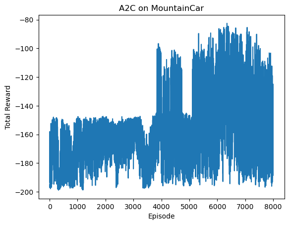
After Training (animation - run in Jupyter for display)

Once Loop Reflect

After Training Position Plot

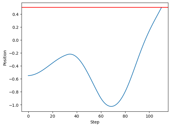
13.9 Key Challenges and Practical Enhancements in RL

Reinforcement learning (RL) faces several core challenges that limit its direct application in real-world engineering systems, as discussed in Brunton and Kutz (Chapter 11) and broader literature. These include the exploration-exploitation dilemma, where the agent must balance trying new actions to discover better strategies (exploration) with leveraging known good actions (exploitation); credit assignment, the difficulty of attributing delayed rewards to earlier actions in long-horizon tasks; and safety, ensuring the agent avoids catastrophic failures during learning. In space engineering contexts, these are amplified: exploration risks could lead to irreversible damage (e.g., satellite collision), credit assignment is critical for multi-step maneuvers like rendezvous, and safety is paramount in high-stakes environments like orbit control. Practical enhancements, such as advanced exploration, constraint-aware methods, and reward engineering, address these to make RL viable for computational engineering practice.

13.9.1 Exploration Strategies

Effective exploration is essential to avoid suboptimal policies trapped in local optima. Basic techniques like random action selection provide initial diversity, but more sophisticated methods balance this with exploitation. ε-greedy strategies select the best-known action (e.g., \( \arg\max_a Q(s,a) \)) with probability 1-ε and a random action from the space \( A \) with probability ε, where ε typically decays over time (e.g., exponentially: ε_{t+1} = ε_t * decay_rate). This ensures early broad sampling, transitioning to exploitation—useful in discrete spaces like mode selection in classical feedback control (Chapter 10), but can be inefficient in high-dimensional continuous spaces due to uniform randomness.

For continuous or stochastic policies, entropy bonuses add a term to the objective proportional to policy entropy H(π(·|s)), encouraging diverse actions. For a Gaussian policy π_θ(u|y) = N(μ_θ(y), σ_θ(y)), entropy H ≈ log(σ) + const, so the loss includes -β H, where β is a coefficient (e.g., 0.01). This prevents policy collapse (σ → 0) and promotes exploration in parameter spaces, akin to regularization in non-linear optimization (Chapter 8). Other techniques include upper confidence bound (UCB), which adds optimism via uncertainty estimates (e.g., Q(s,a) + c √(log t / N(s,a))), or Thompson sampling, sampling actions from posterior beliefs—extending to Bayesian approaches.

Relating to our chapters on global optimization (Chapter 9), exploration in RL mirrors the exploration-exploitation trade-off in derivative-free methods. ε-greedy resembles random search or perturbation in evolutionary strategies, where initial randomness explores the feasible set \( \mathcal{X} \), then focuses on promising regions. Entropy bonuses parallel diversity maintenance in genetic algorithms (e.g., mutation rates) or acquisition functions in Bayesian optimization (e.g., expected improvement balancing mean and variance). In both RL and global optimization, these prevent premature convergence to local minima, crucial for non-convex problems like non-linear programming with parameters p (Chapter 8).

For a basic Python visualization, below is a demo on a multi-armed bandit problem (simplified RL with fixed s, multiple a). It compares ε-greedy (decaying ε) and a constant-entropy-like strategy (via softmax temperature τ, analogous to entropy bonus). The plot shows cumulative regret (suboptimality) over pulls, illustrating better exploration leading to lower regret.

import numpy as np
import matplotlib.pyplot as plt

# Multi-armed bandit: 5 arms with true means (rewards)
true_means = [0.1, 0.5, 0.9, 0.3, 0.7]  # Best arm: 2 (0.9)
num_arms = len(true_means)
num_pulls = 1000

def pull_arm(arm):
    return np.random.normal(true_means[arm], 1.0)  # Noisy rewards

# ε-greedy strategy
def epsilon_greedy(Q, epsilon):
    if np.random.rand() < epsilon:
        return np.random.randint(num_arms)
    return np.argmax(Q)

# Softmax (entropy-like) strategy
def softmax_select(Q, tau=1.0):
    probs = np.exp(Q / tau) / np.sum(np.exp(Q / tau))
    return np.random.choice(num_arms, p=probs)

# Run simulation for a strategy
def simulate(strategy, **kwargs):
    Q = np.zeros(num_arms)
    counts = np.zeros(num_arms)
    rewards = []
    regret = []
    cumulative_regret = 0
    epsilon = 0.1  # Initial for ε-greedy
    for t in range(1, num_pulls + 1):
        if strategy == 'epsilon_greedy':
            arm = epsilon_greedy(Q, epsilon)
            epsilon *= 0.995  # Decay
        else:  # softmax
            tau = kwargs['initial_tau'] / np.log(t + 1)  # Decaying temperature for entropy
            arm = softmax_select(Q, tau)
        reward = pull_arm(arm)
        counts[arm] += 1
        Q[arm] += (reward - Q[arm]) / counts[arm]
        rewards.append(reward)
        instant_regret = max(true_means) - true_means[arm]
        cumulative_regret += instant_regret
        regret.append(cumulative_regret)
    return regret

# Simulate and plot
regret_eg = simulate('epsilon_greedy')
regret_soft = simulate('softmax', initial_tau=5.0)  # High initial entropy

plt.plot(regret_eg, label='ε-Greedy (Decaying ε)')
plt.plot(regret_soft, label='Softmax (Decaying τ ~ Entropy Bonus)')
plt.xlabel('Pulls')
plt.ylabel('Cumulative Regret')
plt.title('Exploration Strategies in Multi-Armed Bandit')
plt.legend()
plt.show()

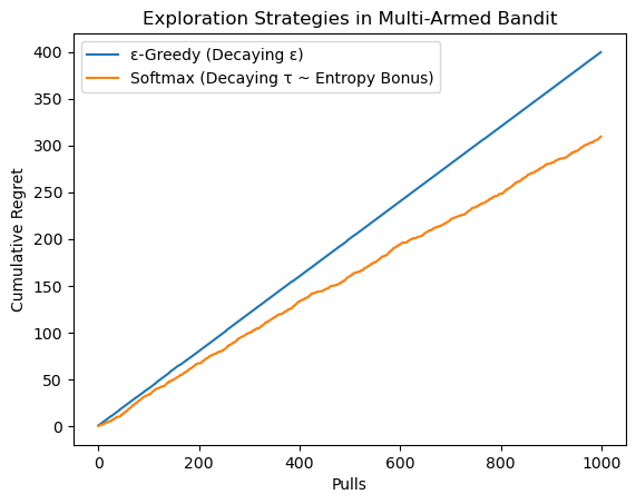
13.9.2 Safety Envelopes and Constraint Handling

Safety is a critical barrier in RL for engineering, where trial-and-error can cause physical harm or mission failure. Safe RL concepts incorporate constraints into learning, such as through constrained MDPs (CMDPs), where the policy optimizes returns subject to cost constraints (e.g., \( \mathbb{E}[C] \leq c \), with C as safety costs like collision risk). Techniques like Lagrangian relaxation treat constraints as penalties in the objective, or use safety shields (e.g., model-based verifiers) to override unsafe actions. In space applications, this aligns with robust control (Chapter 11), ensuring policies respect feasible sets \( \mathcal{Y} \) (e.g., avoiding deorbiting due to excessive thrust) while handling parameters \( \mathbf{p} \) like uncertain disturbances.

13.9.3 Reward Shaping and Curriculum Learning

Reward shaping modifies the sparse MDP reward R to include dense guidance signals without changing optimal policies, using potential-based shaping: \( \tilde{R}(s,a,s') = R(s,a,s') + \gamma \Phi(s') - \Phi(s) \), where \( \Phi \) is a potential function (e.g., distance to goal). This accelerates learning in long-horizon tasks by providing intermediate feedback. Curriculum learning progressively increases task difficulty, starting with easy variants (e.g., shorter horizons or simpler dynamics) and ramping up, mimicking staged simulations in engineering (Chapters 4-6). In space, these enable efficient training for complex maneuvers, like gradual introduction of perturbations \( \mathbf{p} \).

Example: GridWorld shaling

Below is a simple example of reward shaping on a toy GridWorld env (similar to Section 13.5), using Q-learning with/without shaping to show faster convergence. The potential \( \Phi(s) = -\|s - goal\| \) encourages goal proximity. Enhanced visualizations include policy arrows on the grid (showing learned actions) and value heatmaps (max Q per state), connecting the reward changes to policy improvements—e.g., shaped policies exhibit more directed paths.

import numpy as np
import matplotlib.pyplot as plt
from matplotlib.patches import FancyArrowPatch

# Toy GridWorld: 5x5, start (0,0), goal (4,4), actions up/down/left/right
class GridWorld:
    def __init__(self, size=5):
        self.size = size
        self.start = (0, 0)
        self.goal = (4, 4)

    def step(self, state, action):
        x, y = state
        if action == 0: y = min(y + 1, self.size - 1)  # up
        elif action == 1: y = max(y - 1, 0)  # down
        elif action == 2: x = max(x - 1, 0)  # left
        elif action == 3: x = min(x + 1, self.size - 1)  # right
        next_state = (x, y)
        reward = 1 if next_state == self.goal else -1
        done = next_state == self.goal
        return next_state, reward, done

# Q-Learning with optional shaping
def q_learning_with_shaping(shaping=False, episodes=500, alpha=0.1, gamma=0.99, epsilon=0.1):
    env = GridWorld()
    Q = np.zeros((env.size, env.size, 4))  # States x,y; 4 actions
    rewards = []
    for ep in range(episodes):
        state = env.start
        total_reward = 0
        done = False
        while not done:
            if np.random.rand() < epsilon:
                action = np.random.randint(4)
            else:
                action = np.argmax(Q[state])
            next_state, reward, done = env.step(state, action)
            if shaping:
                phi = -np.sum(np.abs(np.array(state) - np.array(env.goal)))  # Manhattan potential
                phi_next = -np.sum(np.abs(np.array(next_state) - np.array(env.goal)))
                reward += gamma * phi_next - phi
            best_next = np.max(Q[next_state])
            Q[state[0], state[1], action] += alpha * (reward + gamma * best_next - Q[state[0], state[1], action])
            state = next_state
            total_reward += reward
        rewards.append(total_reward)
    return rewards, Q

# Visualization: Policy arrows and value heatmap
def visualize_policy_and_values(Q, title, env):
    policy = np.argmax(Q, axis=2)
    values = np.max(Q, axis=2)

    fig, axs = plt.subplots(1, 2, figsize=(12, 5))

    # Policy grid
    ax = axs[0]
    ax.set_title(f'Policy: {title}')
    ax.grid(True)
    ax.set_xlim(0, env.size)
    ax.set_ylim(0, env.size)
    ax.set_xticks(np.arange(env.size + 1))
    ax.set_yticks(np.arange(env.size + 1))
    arrows = [(0, 0.3), (0, -0.3), (-0.3, 0), (0.3, 0)]  # up, down, left, right
    for x in range(env.size):
        for y in range(env.size):
            if (x, y) == env.goal:
                ax.text(x + 0.5, y + 0.5, 'Goal', ha='center', va='center')
                continue
            a = policy[x, y]
            dx, dy = arrows[a]
            ax.add_patch(FancyArrowPatch((x + 0.5 - dx/2, y + 0.5 - dy/2), (x + 0.5 + dx/2, y + 0.5 + dy/2),
                                         arrowstyle='->', mutation_scale=15, color='blue'))

    # Value heatmap
    im = axs[1].imshow(values.T, cmap='viridis', origin='lower')
    axs[1].set_title(f'Values: {title}')
    plt.colorbar(im, ax=axs[1])
    axs[1].set_xlabel('X')
    axs[1].set_ylabel('Y')

    plt.show()

# Run and plot rewards
rewards_base, Q_base = q_learning_with_shaping(shaping=False)
rewards_shaped, Q_shaped = q_learning_with_shaping(shaping=True)

plt.plot(rewards_base, label='Baseline')
plt.plot(rewards_shaped, label='With Shaping')
plt.xlabel('Episode')
plt.ylabel('Total Reward')
plt.title('Reward Shaping Demo on Toy GridWorld')
plt.legend()
plt.show()

# Visualize policies and values
env = GridWorld()  # For reference
visualize_policy_and_values(Q_base, 'Baseline', env)
visualize_policy_and_values(Q_shaped, 'With Shaping', env)

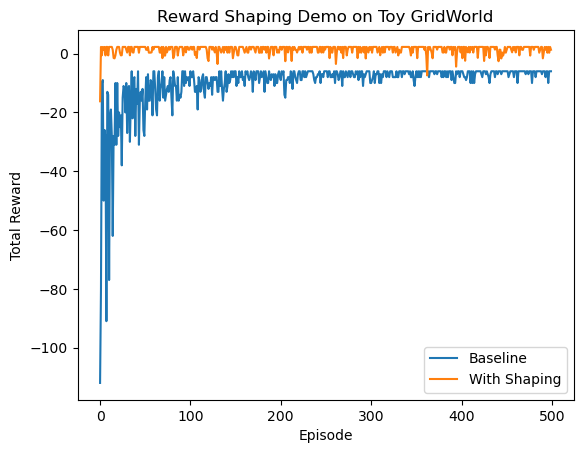
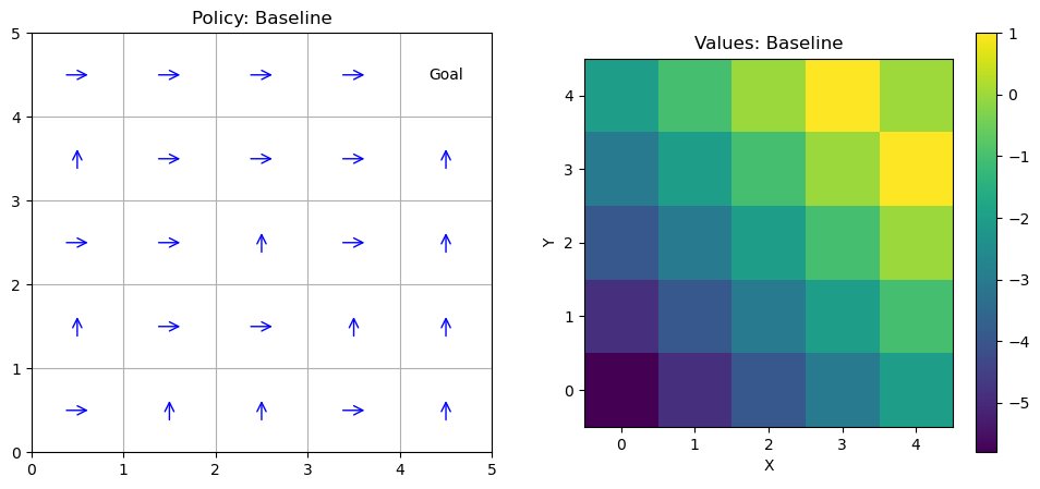
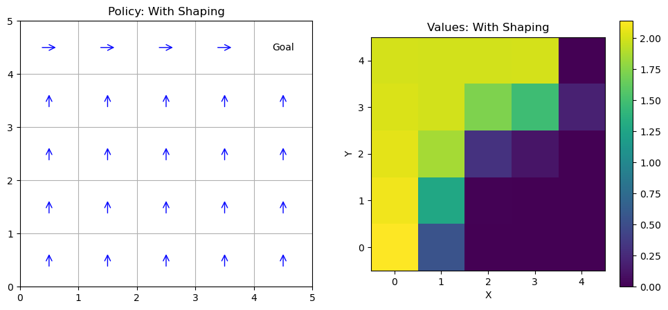
13.10 Summary & Roadmap to Chapter 14

This chapter has introduced the foundations of reinforcement learning (RL), with methods categorized along key dimensions: model-based (explicit dynamics like \( \dot{\mathbf{y}} = \mathbf{f}(\mathbf{y}, \mathbf{u}) \)) vs. model-free (data-driven); gradient-based (using \( \nabla \)) vs. gradient-free (derivative-free, tying to Chapter 9); and on-policy (data from current policy) vs. off-policy (reusable data). These build on earlier course topics, such as dynamic systems (Chapters 1-3), simulation (Chapters 4-6), and optimization (Chapters 7-9), extending to control under uncertainty (Chapters 10-12). Strengths include scalability to non-linear, high-dimensional problems like chaotic dynamics, while weaknesses involve sample inefficiency and lack of guarantees compared to classical methods like LQR. Looking ahead, Chapter 14 applies these to RL-based orbit station-keeping, where an agent optimizes thrust \( \mathbf{u} \) to maintain satellite position \( \mathbf{y} \) amid perturbations \( \mathbf{p} \) (e.g., drag, \( J_2 \)), demonstrating real-time adaptation in space engineering.

13.10.1 Method Comparison Table

The table below summarizes key RL methods from the Brunton and Kutz categorization, highlighting their classifications, strengths, and weaknesses in the context of computational engineering.

Method	Categorization (Model-Based/Free, Gradient-Based/Free, On/Off-Policy)	Strengths	Weaknesses
Dynamic Programming (DP)	Model-based, Gradient-free (value iteration), On-policy (policy iteration)	Exact optimality in known MDPs; efficient for small, discrete spaces (e.g., quantized control modes).	Requires full model knowledge; curse of dimensionality in high-DOF systems like continuum mechanics (Chapter 6).
Monte-Carlo (MC)	Model-free, Gradient-free (tabular), On-policy (with ε-greedy)	Unbiased estimates from full episodes; simple for episodic tasks like simulations (Chapter 4).	High variance from long horizons; inefficient for continuing tasks or real-time control (e.g., orbit adjustments).
Temporal-Difference (TD)	Model-free, Gradient-free (tabular Q/SARSA), On/Off-policy	Bootstrapping reduces variance; online learning for dynamic systems (Chapter 5 ODE/DAE).	Bias in early estimates; sensitive to hyperparameters like α in non-linear environments (Chapter 3 chaos).
Deep Q-Networks (DQN)	Model-free, Gradient-based (neural approx.), Off-policy	Scales to high-dimensional states (e.g., sensor data); experience replay stabilizes training.	Overestimation bias; computationally intensive for deep nets, similar to non-linear optimization costs (Chapter 8).
Policy Gradients (REINFORCE)	Model-free, Gradient-based, On-policy	Direct policy optimization for continuous actions Π; handles stochasticity.	High variance without baselines; slow convergence in long-horizon problems like multi-step maneuvers.
Actor-Critic (A2C/A3C)	Model-free, Gradient-based, On-policy (A2C)	Lower variance via critic bootstrapping; parallelizable for faster training (A3C).	Still sensitive to hyperparameters; actor-critic divergence in unstable dynamics (e.g., non-linear control, Chapter 12).

13.10.2 Transition to Space Applications

The foundations covered here: MDPs, value/policy iteration, TD methods, deep approximations, and policy gradients, provide a toolkit for tackling real engineering problems where models are incomplete or environments stochastic. In space applications, these enable agents to learn adaptive policies for tasks like attitude control (mapping observations \( \mathbf{y} \) to thrusts \( \mathbf{u} \)) amid uncertainties \( \mathbf{p} \) (e.g., solar radiation), bridging classical methods (e.g., PID/LQR from Chapters 10-11) with data-driven robustness. Unlike deterministic simulations (Chapters 4-6), RL handles partial observability and non-linearity (Chapter 3), optimizing over feasible sets \( \mathcal{Y} \) without explicit programming. Chapter 14 applies this to RL-based orbit station-keeping, where an agent minimizes fuel while maintaining position against perturbations, showcasing hierarchical RL and edge compute for onboard autonomy: extending model-predictive control (Chapter 12) to learning-based paradigms.

Further reading

This section provides key references for deeper study, including textbooks, seminal papers, and resources tied to each subsection. The primary textbook for RL foundations is Sutton and Barto’s Reinforcement Learning: An Introduction (2nd ed., 2018), which covers most topics comprehensively. Brunton and Kutz (Chapter 11) offers a data-driven perspective linking RL to dynamical systems. References are selected for their relevance to computational engineering, emphasizing numerical methods and applications.

RL applications in space engineering:

• Reinforcement learning-based station keeping using relative orbital elements. Available at: https://www.sciencedirect.com/science/article/pii/S0273117725004533.

• Reinforcement learning-based station keeping using relative orbital elements. Available at: https://www.diva-portal.org/smash/get/diva2:1966369/FULLTEXT02.

• Deep reinforcement learning for station keeping on near rectilinear halo orbits. Available at: https://www.merl.com/publications/docs/TR2023-098.pdf.

• Meta-Reinforcement Learning for Spacecraft Proximity Operations Guidance and Control in Cislunar Space. Available at: https://hanspeterschaub.info/PapersPrivate/Fereoli2025.pdf.

• Autonomous Six-Degree-of-Freedom Spacecraft Docking with Rotating Targets via Reinforcement Learning. Available at: https://dspace.mit.edu/bitstream/handle/1721.1/145412/2008.03215.pdf?isAllowed=y&sequence=2.

• Revisiting Space Mission Planning: A Reinforcement Learning-Guided Approach for Multi-Debris Rendezvous. Available at: https://arxiv.org/html/2409.16882v1.

• An improved path planning and tracking control method for planetary exploration rovers on rough terrain. Available at: https://www.sciencedirect.com/science/article/pii/S2667379725000105.

• Hopping path planning in uncertain environments for planetary exploration. Available at: https://link.springer.com/article/10.1186/s40648-022-00219-7.

• Learning-Based End-to-End Path Planning for Lunar Rovers with Safety Constraints. Available at: https://pmc.ncbi.nlm.nih.gov/articles/PMC7866010.

• Review of Autonomous Space Robotic Manipulators for On-Orbit Servicing and Active Debris Removal. Available at: https://spj.science.org/doi/10.34133/space.0291.

• Review of machine learning in robotic grasping control in space application. Available at: https://www.sciencedirect.com/science/article/pii/S009457652400211X.

• Learning Dexterous Manipulation for a Soft Robotic Hand from Human Demonstration. Available at: https://arxiv.org/abs/1603.06348.

Section specific references:

13.1 Motivation: From Classical & Optimal Control to Learning-Based Control

• Sutton, R. S., & Barto, A. G. (2018). Reinforcement Learning: An Introduction (2nd ed.). MIT Press. (Chapters 1-2: Bridges control theory to RL, highlighting uncertainty handling.)

• Bertsekas, D. P. (2019). Reinforcement Learning and Optimal Control. Athena Scientific. (Seminal textbook comparing RL to optimal control, with engineering examples like MPC vs. RL.)

• Levine, S. (2018). “Reinforcement Learning and Control as Probabilistic Inference: Tutorial and Review.” arXiv preprint arXiv:1805.00909. (Paper relating RL to probabilistic control, relevant for space applications.)

13.1.1 When RL Shines in Engineering

• Brunton, S. L., & Kutz, J. N. (2019). Data-Driven Science and Engineering (Chapter 11). Cambridge University Press. (Discusses RL in engineering contexts where models are incomplete.)

• Recht, B. (2019). “A Tour of Reinforcement Learning: The View from Continuous Control.” Annual Review of Control, Robotics, and Autonomous Systems, 2, 253-279. (Review paper on RL in continuous control, with space-relevant examples like robotics.)

13.1.2 Limitations and Practical Considerations

• Dulac-Arnold, G., et al. (2021). “Challenges of Real-World Reinforcement Learning: Definitions, Benchmarks and Analysis.” Machine Learning, 110(9), 2419-2468. (Paper on RL challenges in practice, including sample inefficiency and safety.)

• Garcia, J., & Fernández, F. (2015). “A Comprehensive Survey on Safe Reinforcement Learning.” Journal of Machine Learning Research, 16(1), 1437-1480. (Survey on safety issues, linking to engineering constraints.)

13.2 Overview of Reinforcement Learning Methods

• Brunton & Kutz (Chapter 11): Core categorization (Figure 11.3) of RL methods.

• Kaelbling, L. P., Littman, M. L., & Moore, A. W. (1996). “Reinforcement Learning: A Survey.” Journal of Artificial Intelligence Research, 4, 237-285. (Seminal survey paper on early RL categorizations.)

13.2.1 Model-Based vs. Model-Free RL

• Sutton & Barto (2018): Chapters 8-9 on model-based vs. model-free.

• Deisenroth, M. P., & Rasmussen, C. E. (2011). “PILCO: A Model-Based Policy Search Method.” Proceedings of the 28th International Conference on Machine Learning. (Seminal paper on model-based RL with Gaussian processes.)

13.2.2 Gradient-Based vs. Gradient-Free Methods

• Schulman, J., et al. (2015). “Trust Region Policy Optimization.” Proceedings of the 32nd International Conference on Machine Learning. (Paper on gradient-based TRPO, linking to optimization.)

• Hansen, N. (2006). “The CMA Evolution Strategy: A Comparing Review.” In Towards a New Evolutionary Computation (pp. 75-102). Springer. (On gradient-free evolutionary strategies.)

13.2.3 On-Policy vs. Off-Policy Learning

• Sutton & Barto (2018): Chapter 5 on on/off-policy TD methods.

• Precup, D., Sutton, R. S., & Singh, S. (2000). “Eligibility Traces for Off-Policy Policy Evaluation.” Proceedings of the 17th International Conference on Machine Learning. (Seminal on off-policy with traces.)

13.3 Markov Decision Processes (MDPs) – The Mathematical Framework

• Puterman, M. L. (1994). Markov Decision Processes: Discrete Stochastic Dynamic Programming. Wiley. (Classic textbook on MDPs.)

• Bellman, R. (1957). “A Markovian Decision Process.” Journal of Mathematics and Mechanics, 6(5), 679-684. (Seminal paper introducing MDPs.)

13.4 Policies, Value Functions, and Bellman Equations

• Sutton & Barto (2018): Chapters 3-4 on policies, values, and Bellman equations.

• Bellman, R. (1957). Dynamic Programming. Princeton University Press. (Original work on Bellman equations.)

13.5 Dynamic Programming – Solving Known MDPs

• Bertsekas, D. P. (2012). Dynamic Programming and Optimal Control (Vol. 1, 4th ed.). Athena Scientific. (Detailed on DP methods.)

• Howard, R. A. (1960). Dynamic Programming and Markov Processes. MIT Press. (Early work on policy iteration.)

13.6 Model-Free Methods: Monte-Carlo and Temporal-Difference Learning

• Sutton & Barto (2018): Chapters 5-6 on MC and TD.

• Watkins, C. J. C. H., & Dayan, P. (1992). “Q-Learning.” Machine Learning, 8(3-4), 279-292. (Seminal paper on Q-learning.)

13.7 Function Approximation and Deep Reinforcement Learning

• Mnih, V., et al. (2015). “Human-Level Control through Deep Reinforcement Learning.” Nature, 518(7540), 529-533. (Seminal DQN paper.)

• Tsitsiklis, J. N., & Van Roy, B. (1997). “An Analysis of Temporal-Difference Learning with Function Approximation.” IEEE Transactions on Automatic Control, 42(5), 674-690. (On function approximation convergence.)

13.8 Policy Gradient Methods and Actor-Critic

• Sutton, R. S., et al. (1999). “Policy Gradient Methods for Reinforcement Learning with Function Approximation.” Advances in Neural Information Processing Systems, 12. (Seminal on policy gradients.)

• Schulman, J., et al. (2017). “Proximal Policy Optimization Algorithms.” arXiv preprint arXiv:1707.06347. (PPO paper, extending actor-critic.)

13.9 Key Challenges and Practical Enhancements in RL

• Brunton & Kutz (Chapter 11): Discusses challenges like exploration and credit assignment.

• Amodei, D., et al. (2016). “Concrete Problems in AI Safety.” arXiv preprint arXiv:1606.06565. (On safety and exploration challenges.)

13.9.1 Exploration Strategies

• Auer, P. (2002). “Using Confidence Bounds for Exploitation-Exploration Trade-offs.” Journal of Machine Learning Research, 3, 397-422. (On UCB exploration.)

• Osband, I., et al. (2016). “Deep Exploration via Bootstrapped DQN.” Advances in Neural Information Processing Systems, 29. (On deep exploration techniques.)

13.9.2 Safety Envelopes and Constraint Handling

• García & Fernández (2015): Survey on safe RL.

• Achiam, J., et al. (2017). “Constrained Policy Optimization.” Proceedings of the 34th International Conference on Machine Learning. (On constrained MDPs.)

13.9.3 Reward Shaping and Curriculum Learning

• Ng, A. Y., Harada, D., & Russell, S. (1999). “Policy Invariance Under Reward Transformations: Theory and Application to Reward Shaping.” Proceedings of the 16th International Conference on Machine Learning. (Seminal on potential-based shaping.)

• Bengio, Y., et al. (2009). “Curriculum Learning.” Proceedings of the 26th International Conference on Machine Learning. (Seminal on curriculum learning.)

13.10 Summary & Roadmap to Chapter 14

• Izzo, D., et al. (2019). “A Survey on Artificial Intelligence Trends in Spacecraft Guidance Dynamics and Control.” Astrodynamics, 3(4), 287-299. (Previewing RL in space, linking to Chapter 14.)