Chapter 12 Control III – model-predictive & non-linear#
12.1 Introduction#
Model Predictive Control (MPC) builds on the optimal control concepts from previous chapters (e.g., LQR in Chapter 11) by incorporating predictions, optimization, and constraints in real-time. This chapter provides a concise overview, focusing on core definitions, descriptions, and simple code examples. We’ll connect MPC to reinforcement learning (RL) in Chapter 13, where MPC-like planning inspires model-based RL methods.
12.2 MPC Definition and Description#
MPC is a feedback control strategy that:
Uses a dynamic model to predict the system’s future states over a finite prediction horizon (e.g., \( N \) steps).
Solves an optimization problem at each time step to find the optimal sequence of control inputs that minimizes a cost function (e.g., quadratic error to a setpoint) while respecting constraints (e.g., input limits, state bounds).
Applies only the first control input from the sequence.
Repeats the process at the next time step with updated measurements (receding horizon).
Key advantages:
Handles multi-input multi-output (MIMO) systems, constraints, and non-linearities explicitly.
Bridges classical control (e.g., PID, LQR) with optimization-based methods.
For a discrete-time system \( \mathbf{y}_{k+1} = \mathbf{A} \mathbf{y}_k + \mathbf{B} \mathbf{u}_k \), the MPC optimization problem is typically:
Subject to dynamics, \( \mathbf{y}_{k+i} = \mathbf{A} \mathbf{y}_{k+i-1} + \mathbf{B} \mathbf{u}_{k+i-1} \), and constraints (e.g., \( |\mathbf{u}| \leq \mathbf{u}_{\max} \)).
12.3 Linear MPC Example
We’ll simulate a simple double-integrator system (e.g., position control): \( \dot{\mathbf{y}} = \begin{bmatrix} 0 & 1 \\ 0 & 0 \end{bmatrix} \mathbf{y} + \begin{bmatrix} 0 \\ 1 \end{bmatrix} u \), discretized with time step \( \Delta t = 0.1 \).
Use scipy.optimize.minimize for the quadratic cost (approximates QP for linear cases).
import numpy as np
from scipy.optimize import minimize
import matplotlib.pyplot as plt

# System matrices (discretized double integrator)
dt = 0.1
A = np.array([[1, dt], [0, 1]])
B = np.array([[0.5*dt**2], [dt]])
n_states = 2
n_inputs = 1

# MPC parameters
N = 10  # Prediction horizon
Q = np.eye(n_states)  # State cost
R = 0.1 * np.eye(n_inputs)  # Input cost
y_ref = np.array([1.0, 0.0])  # Setpoint: position=1, velocity=0
u_min, u_max = -1.0, 1.0  # Input constraints

def mpc_cost(u_seq, y0):
    """Quadratic cost function for optimization."""
    cost = 0.0
    y = y0.reshape(-1, 1)  # Ensure column vector
    for i in range(N):
        u = u_seq[i*n_inputs:(i+1)*n_inputs].reshape(-1, 1)
        y = A @ y + B @ u
        state_err = y - y_ref.reshape(-1, 1)
        cost += (state_err.T @ Q @ state_err).item() + (u.T @ R @ u).item()
    return cost

# Simulation
T = 100  # Time steps
y_traj = np.zeros((n_states, T+1))
u_traj = np.zeros((n_inputs, T))
y = np.array([0.0, 0.0])  # Initial state
y_traj[:, 0] = y

for t in range(T):
    # Optimize: initial guess (warm-start: shift previous solution or zeros)
    u_guess = np.zeros(N * n_inputs)
    bounds = [(u_min, u_max)] * (N * n_inputs)
    res = minimize(mpc_cost, u_guess, args=(y,), bounds=bounds)
    u_seq_opt = res.x
    u = u_seq_opt[:n_inputs]  # Apply first input
    y = (A @ y.reshape(-1, 1) + B @ u.reshape(-1, 1)).flatten()
    y_traj[:, t+1] = y
    u_traj[:, t] = u

# Plot
plt.figure(figsize=(10, 4))
plt.subplot(1, 2, 1)
plt.plot(y_traj[0], label='Position')
plt.plot([0, T], [y_ref[0], y_ref[0]], 'r--', label='Ref')
plt.legend(); plt.title('State Trajectory')
plt.subplot(1, 2, 2)
plt.plot(u_traj[0], label='Input')
plt.plot([0, T], [u_max, u_max], 'r--'); plt.plot([0, T], [u_min, u_min], 'r--')
plt.legend(); plt.title('Control Input')
plt.show()
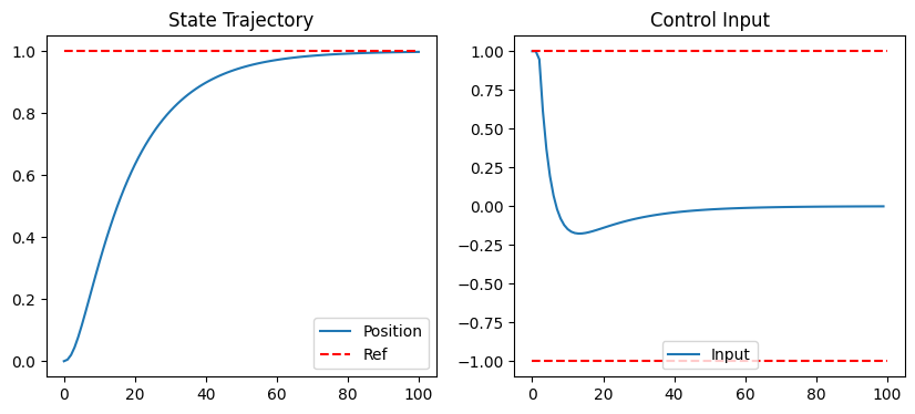
This code solves the MPC problem at each step, applying constraints via bounds. Warm-starting can be added by shifting u_seq_opt from the previous step as u_guess (e.g., u_guess = np.concatenate((u_seq_opt[n_inputs:], np.zeros(n_inputs)))).
12.4 Nonlinear MPC and Successive Linearization#
For nonlinear systems (e.g., \( \mathbf{y}_{k+1} = \mathbf{f}(\mathbf{y}_k, \mathbf{u}_k) \)), the optimization becomes non-convex. Use scipy.optimize.minimize with methods like ‘SLSQP’ for constraints.
Successive linearization: At each MPC step, linearize the nonlinear model around the current state/trajectory, solve the linear MPC, and iterate (e.g., 2-5 times) for refinement.
Warm-start: Use the previous optimal sequence as the initial guess to speed up convergence.
Constraint handling: Include state/input constraints directly in the optimizer (e.g., via constraints arg in minimize).
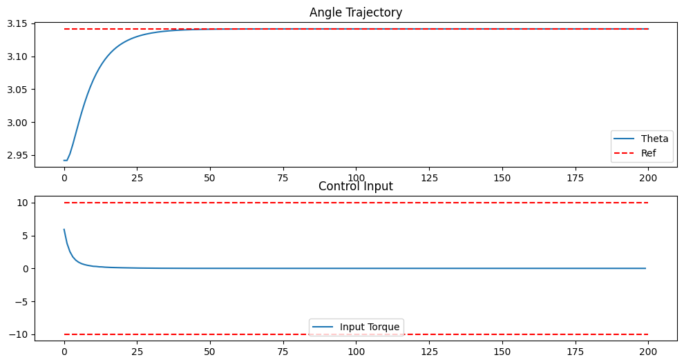
Example: nonlinear MPC
Consider the nonlinear pendulum: \( \frac{d^2 \theta}{dt^2} = -\frac{g}{l} \sin(\theta) + \frac{1}{ml^2} u \)):
import numpy as np
from scipy.optimize import minimize
import matplotlib.pyplot as plt

# Nonlinear pendulum parameters
g, l, m = 9.81, 1.0, 1.0
dt = 0.05
y_ref = np.array([np.pi, 0.0])  # Inverted position, zero velocity
N = 10  # Prediction horizon
Q = np.diag([10.0, 1.0])  # State weights: more on angle
R = 0.01  # Input weight (small to allow larger torques)
u_min, u_max = -10.0, 10.0  # Input constraints

def nonlinear_dynamics(y, u):
    theta, omega = y
    dtheta_dt = omega
    d2theta_dt2 = - (g/l) * np.sin(theta) + (1/(m*l**2)) * u
    return np.array([theta + dt * dtheta_dt, omega + dt * d2theta_dt2])

def nl_mpc_cost(u_seq, y0):
    cost = 0.0
    y = y0.copy()
    for i in range(N):
        u = u_seq[i]
        y = nonlinear_dynamics(y, u)
        cost += (y - y_ref) @ Q @ (y - y_ref) + R * u**2
    return cost

# Simulation
T = 200  # Time steps (longer for stabilization)
y_traj = np.zeros((2, T+1))
u_traj = np.zeros(T)
y = np.array([np.pi - 0.2, 0.0])  # Initial state: slightly off inverted
y_traj[:, 0] = y
prev_u_seq = np.zeros(N)  # For warm-start

for t in range(T):
    u_guess = prev_u_seq
    bounds = [(u_min, u_max)] * N
    res = minimize(nl_mpc_cost, u_guess, args=(y,), method='SLSQP', bounds=bounds)
    u_seq_opt = res.x
    u = u_seq_opt[0]
    y = nonlinear_dynamics(y, u)
    y_traj[:, t+1] = y
    u_traj[t] = u
    # Warm-start: shift sequence and append zero
    prev_u_seq = np.concatenate((u_seq_opt[1:], [0.0]))

# Plot
plt.figure(figsize=(12, 6))
plt.subplot(2, 1, 1)
plt.plot(y_traj[0], label='Theta')
plt.plot([0, T], [y_ref[0], y_ref[0]], 'r--', label='Ref')
plt.legend(); plt.title('Angle Trajectory')
plt.subplot(2, 1, 2)
plt.plot(u_traj, label='Input Torque')
plt.plot([0, T], [u_max, u_max], 'r--'); plt.plot([0, T], [u_min, u_min], 'r--')
plt.legend(); plt.title('Control Input')
plt.show()
(Optional) For Jacobians, use sympy to compute linearizations symbolically:
import sympy as sp

theta, omega, u = sp.symbols('theta omega u')
f = sp.Matrix([omega, - (g/l) * sp.sin(theta) + (1/(m*l**2)) * u])
A_sym = f.jacobian([theta, omega])
B_sym = f.jacobian([u])
# Lambdify for numerical eval: A = sp.lambdify((theta, omega, u), A_sym)
12.5 (Optional) Intro to Data-Driven MPC: SINDy / DMDc#
For systems without known models, use data-driven methods:
SINDy (Sparse Identification of Nonlinear Dynamics): Fits sparse nonlinear ODEs from data via regression. DMDc (Dynamic Mode Decomposition with Control): Extends DMD for controlled systems, estimating A/B matrices.
Use these to learn models for MPC (e.g., via scipy regression). Skip for now; see literature for integration with MPC.
12.6 Connection to Reinforcement Learning (Chapter 13)#
MPC is a form of model-based optimal control with finite horizons and explicit models/constraints. RL (Chapter 13) extends this to:
Infinite horizons via value/policy functions. Learning models/rewards from data (model-free vs. model-based RL, where MPC inspires planning in model-based RL like Dyna or AlphaZero). Handling uncertainty (e.g., stochastic MDPs) with safety (similar to MPC constraints via reward shaping).
In Chapter 14’s orbit station-keeping, RL agents can be viewed as “learning MPC” policies for complex, nonlinear dynamics. For further reading: “Model Predictive Control” by Rawlings et al.; connect to RL via “Reinforcement Learning: An Introduction” by Sutton & Barto.