Chapter 1: Model classification I – building blocks

“A problem well stated is a problem half-solved.”

— Charles F. Kettering

1 Model classification and structure

1.1 What are models? From toy cathedrals to floating point arithmetic

To measure is to know.

— William Thomson (Lord Kelvin), 1883

While we often think of models as mathematical equations, the mathematication of nature is a relatively recent development in the history of science and engineering. Models have existed in various forms for centuries, evolving from physical constructions to modern abstract mathematical representations. Some historical milestones in the practice of modelling include:

1.2 Medieval (Physical (literal) models)

• Medieval master-builders often erected stick-and-string scale models of vaults and domes to study thrust lines.

• Brunelleschi’s herringbone brick pattern for the Florence Duomo (1430s) was tested on a wooden mock-up before construction.

• Siege engineers constructed full-scale or prototyped trebuchets, powerful counterweight-based siege engines, to test projectile trajectories and structural integrity, embodying principles of leverage and force balance in mechanical warfare. This practice marks the French-root origin of the modern word “engineer” (from Old French “engigneor,” meaning one who designs or operates siege engines) and the engineering profession, which began in military contexts.

• These tangible artefacts embodied the equilibrium of forces as a precursor to statics theory, itself a precursor to more complex mathematized models of nature such as Newtonian Physics.

1.3 Early mathematical models (smooth models)

• Jordanus de Nemore (13 th c.) treated levers and centres of gravity with geometric abstraction.

• Johannes Kepler (early 1600s) formulated the three laws of planetary motion based on detailed astronomical observations from Tycho Brahe, providing the first precise mathematical description of elliptical orbits and laying empirical foundations for celestial mechanics and data driven modelling.

• Galileo Galilei (1600s) introduced the concept of inertia and the first mathematical model of motion, laying the groundwork for classical mechanics.

• Isaac Newton’s Principia (1687) ushered in the era of mathematical physics, introducing calculus to describe motion and forces.

• Leonhard Euler (1740s) and D’Alembert introduced differential equations to describe beams, fluids, and celestial mechanics. Euler’s equation for a buckling column is still taught today.

• Joseph Fourier (1822) developed the analytical theory of heat conduction, introducing Fourier series to solve partial differential equations for heat flow in solids— foundational for engineering thermodynamics.

• Claude-Louis Navier and George Gabriel Stokes (1820s-1840s) formulated the Navier-Stokes equations, providing a mathematical framework for fluid motion essential to aerospace and mechanical engineering.

1.4 Modern, discrete models (numerical models)

• Early hand computations by Isaac Newton, Gottfried Wilhelm Leibniz and others laid the groundwork for numerical methods.

• Lewis Fry Richardson (1922) pioneered numerical weather prediction using finite difference methods on the Navier-Stokes equations, an early engineering application of discretization for fluid dynamics.

• Alexander Hrennikoff and Richard Courant (1940s) introduced the finite element method (FEM) for structural analysis, enabling discrete approximations of continuum problems in civil and aerospace engineering.

• Theodore von Kármán (1930s-1950s) advanced numerical methods in aerodynamics, including boundary layer theory, influencing computational simulations for supersonic flight and rocket design.

• First general purpose high level programming language Konrad Zuse’s Plankalkül (1942), Claude Shannon’s information theory (1948) and von Neumann’s stored-program computer made it routine to encode physics directly in software.

Our focus in this module is on discrete or digital models, which are fundamentally different to both physical and smooth models in a subtle and important way: while smooth mathematical models can often admit exact solutions, discretized models -by contrast- rarely admit exact solutions. This is not only due to numerical errors, but due to the fact that these models live in an entirely different space and number system. E.g. smooth models often have scalar variables represented by real numbers (\(\mathbb{R}^n\)) which is not a computational structure! By contrast models for control systems often rely on a discrete \(\mathbb{Z}^n\) representation of scalar variables arising from inherently discrete measurements in the control loop. For example, floating point artithmetic has a different result compared to what we expect from real number addition:

# Expected result of 0.1 + 0.2 = 0.3 in the real number system
a = 0.1
b = 0.2
c = a + b
print(f"0.1 + 0.2 = {c}")  # Output: 0.30000000000000004 (floating-point error)

0.1 + 0.2 = 0.30000000000000004

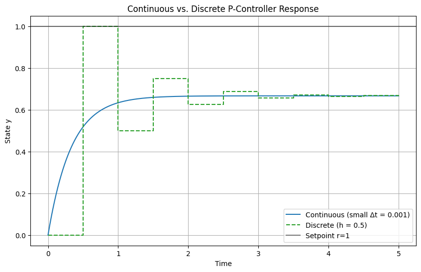
In addition to that we often have to work in a discrete space built on top of the floating point precision number system, for example, modern digital control systems do not sample continuously (unlike, say, traditional pneumatic controllers), therefore they have a worse performance as this simplest case for a proportional controller shows:

import numpy as np
import matplotlib.pyplot as plt

# Parameters
K = 2.0  # Proportional gain
r = 1.0  # Setpoint (step input)
t_end = 5.0  # Simulation end time
y0 = 0.0  # Initial state

# Function for one Euler step: y_next = y + dt * (-y + u), u = K*(r - y)
def euler_step(y, dt, K, r):
    u = K * (r - y)
    return y + dt * (-y + u)

# Simulate "continuous" (small dt = 0.001)
dt_cont = 0.001
n_cont = int(t_end / dt_cont) + 1
t_cont = np.linspace(0, t_end, n_cont)
y_cont = np.zeros(n_cont)
y_cont[0] = y0
for i in range(1, n_cont):
    y_cont[i] = euler_step(y_cont[i-1], dt_cont, K, r)

# Discrete with moderate sampling (h = 0.5, stable but oscillatory)
h_mod = 0.5
n_mod = int(t_end / h_mod) + 1
t_mod = np.linspace(0, t_end, n_mod)
y_mod = np.zeros(n_mod)
y_mod[0] = y0
for i in range(1, n_mod):
    y_mod[i] = euler_step(y_mod[i-1], h_mod, K, r)

# Plot results
plt.figure(figsize=(10, 6))
plt.plot(t_cont, y_cont, label='Continuous (small Δt = 0.001)', color='tab:blue')
plt.step(t_mod, y_mod, where='post', label='Discrete (h = 0.5)', color='tab:green', linestyle='--')
plt.axhline(r, color='black', linestyle='-', label='Setpoint r=1', alpha=0.5)
plt.xlabel('Time')
plt.ylabel('State y')
plt.title('Continuous vs. Discrete P-Controller Response')
plt.legend()
plt.grid(True)
plt.show()

# Demonstrate floating-point accumulation (exaggerated: many steps with tiny dt)
# In real arithmetic, sum should be exactly 1.0; in float, slight error
tiny_dt = 1e-6
num_steps = int(1e6)  # 1 / 1e-6 = 1e6 steps to integrate over t=1
sum_error = 0.0
for _ in range(num_steps):
    sum_error += tiny_dt
print(f"Sum of {num_steps} tiny floats (should be 1.0): {sum_error}")
print(f"Error: {abs(sum_error - 1.0)}")  # Typically ~1e-16 due to float precision

Sum of 1000000 tiny floats (should be 1.0): 1.000000000007918
Error: 7.918110611626616e-12

For the purposes of this course, we will define a model as follows:

Definition: A model is an abstraction which is a deliberate simplification of nature that allows quantitative prediction.

In order to make predictions with computational models, it is essential to correctly classify them in order to find the correct abstracted method for their solutions which in turn is used to predict the outcome of systems such as the dynamics spacecraft, robots, or chemical processes. Later we will study the optimization (design, parameterisation) and control of systems.

---

2 Classification of models

Models admit different structures which can be classified in order to gain better understanding of their properties. Once a model has been classified it becomes easier to compute. Understanding the limitations of state-of-the-art methods used to solve different model types is essential to both model development and computational efficiency of solutions.

When trying to solve your computational problem model classification tells you:

• Which numerical methods will work.

• The expected accuracy and computational cost of solving the system.

• Whether you can exploit powerful results from linear-system theory (superposition, symmetry, modal analysis, controllability, etc.).

2.1 Static vs. dynamic

Models differ in their treatment of time: static models describe systems at equilibrium where time derivatives are zero, focusing on steady-state solutions. Dynamic models incorporate time evolution, capturing transient behaviors and responses to inputs. This classification guides the choice of solvers: algebraic for static, integrators for dynamic—and is vital in fields like spacecraft trajectory planning, where static approximations may suffice for equilibrium orbits but dynamics are essential for maneuvers.

	Static	Dynamic
Abstraction	\(\mathbf{f}(\mathbf{x}) = \mathbf{0}\) (no time derivatives)	\(\frac{d\mathbf{y}}{dt} = \mathbf{f}(\mathbf{y}, \mathbf{x}, t)\) or \(\mathbf{y}(t+1) = \mathbf{f}(\mathbf{y}(t), \mathbf{x})\)
Typical mathematized examples	\(A\mathbf{x} = \mathbf{b}\) (linear system) \(\nabla^2 x = c\) (Poisson’s equation) \(\nabla \cdot (k \nabla T) = 0\) (steady-state heat)	\(\frac{dy}{dt} = -k x\) (exponential decay) \(\frac{d^2y}{dt^2} + \omega^2 x = 0\) (simple harmonic motion) \(\frac{\partial y}{dt} = k \nabla^2 T\) (dynamic heat)
Examples in nature	Truss analysis in civil engineering (equilibrium forces); Steady-state heat conduction in a satellite panel	Launch trajectory optimization (time-varying thrust); Satellite attitude slew maneuver (rotational dynamics over time)

Definition: Let \(\mathcal{x}\) be a state space and \(\mathcal{F}\) a model mapping. The model is static if \(\mathcal{X} : \mathcal{X} \to \mathcal{X}\) does not explicitly depend on time \(t\) and involves no time derivatives (i.e., equilibrium conditions). It is dynamic if \(\mathcal{F} : \mathcal{Y} \times \mathbb{R} \to \mathcal{Y}\) includes time derivatives or discrete time steps, describing evolution over \(t \in \mathbb{R}\) or \(t \in \mathbb{Z}\).

Static problems

Static problems typically arise from modelling physical and chemical systems at equilibrium, where the state does not change over time. These problems can be represented by algebraic equations, differential- or partial differential equations (PDEs) that describe the relationships between variables without involving time derivatives. Examples include structural analysis (statics and strength of materials), heat conduction, and fluid statics. It should be noted that time is not absent in static models, but rather the variables in the equations are not affected by time. For example, financial models may be static in the sense that they do not change over time, but they still involve variables that are functions of time, such as interest rates or stock prices. Such models are important in engineering when optimizing systems for cost saving or computing expected cash flows due to production, maintenance or repairs etc. which accumulate over time.

Static solvers

Static equations are typically solved with root-finding methods, which find the roots of the residual function \(\mathbf{F}(\mathbf{x}) = \mathbf{0}\), where \(\mathbf{F}\) encodes the algebraic system such as a vector of functions. Common numerical methods such as those implemented in scipy include:

Common SciPy-based approaches

Problem type	scipy implementation	Notes
Scalar, nonlinear	scipy.optimize.root_scalar	Bisection, secant, Brent, Ridder …
Vector, nonlinear	scipy.optimize.root scipy.optimize.fsolve	Newton–Krylov, hybr, Levenberg–Marquardt
Least-squares residuals	scipy.optimize.least_squares	Gauss-Newton, trust-region reflective
Fixed-point iteration	scipy.optimize.fixed_point	Finds \(x = f(x)\) directly
Dense linear system	scipy.linalg.solve	\(A\mathbf{x} = \mathbf{b}\) with LU factorisation
Sparse linear system	scipy.sparse.linalg.spsolve	For large, sparse \(A\)

---

The simples example is solving a non-linear single variable equation such as \(f(x) = x^2 - 5 = 0\) using scipy.optimize.root_scalar:

from scipy.optimize import root_scalar

f = lambda x: x**2 - 5

#NOTE: The `lambda` function is a small anonymous function in Python which we will use often for toy examples. The above function is equivalent to:
def f(x):
    return x**2 - 5
# which is often simpler to read for beginners.

sol = root_scalar(f, bracket=[0, 3], method='brentq')

print(f"Root = {sol.root:.6f}")        # ~2.236068 (≈ √5)

Root = 2.236068

Most systems engineers will deal with are multivariate, which is still solved with the same methods, but now the residual function \(\mathbf{F}(\mathbf{x})\) is a vector of functions. The simplest example is solving a linear system of equations such as \(Ax = b\) using scipy.linalg.solve:

import numpy as np
from scipy.linalg import solve

A = np.array([[3.0, 1.0],
              [1.0, 2.0]])
b = np.array([9.0, 8.0])

x = solve(A, b)        # direct LU factorisation
print("x =", x)        # → [2. 3.]

x = [2. 3.]

An important concept in solving complex non-linear models accurately and efficiently is the notion of the Jacobian matrix, which is the matrix of all first-order partial derivatives of the residual function \(\mathbf{F}(\mathbf{x})\). The Jacobian is used to improve convergence in iterative methods such as Newton’s method and will be discussed in more detail in “Week 4: Simulation I – algebraic systems”

Example: Steady-state heat conduction on a square plate

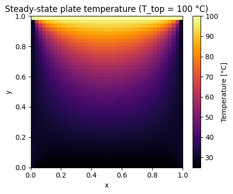
Below is a more complex model of the Laplace equation \(\nabla\!\cdot\!\bigl(k\nabla T\bigr)=0\) with Dirichlet boundary condition. Such complex systems involving gradients can still be solved with the same root solver abstractions. It’s important to get comfortable with the geometric meaning of operators like \(\nabla\) for which static models become a great tool to gain deeper understanding for yourself with respect to its effect on scalar and vector fields. In the demonstration below you can interactively change the temperature on the top edge of the plate and see how the steady-state temperature scalar field changes.

The solution is computed using a root-finding method that iteratively solves for the temperature at each grid point until convergence is reached. Later we will learn a lot about how operators such as \(\nabla\) can be discretized, analyzed for stability and solved efficiently using numerical methods such as finite difference, finite element or finite volume methods. The example below is a simple finite difference method that uses the average of the neighbouring grid points to compute the temperature at each point in the grid. For now we can derive a simplified version of the Laplace equation using finite central differences by exploiting the fact that the right hand side of the eqaution is zero (no internal heat generation). The derivation in 2D is as follows:

\[\nabla\!\cdot\!\bigl(k\nabla T\bigr) = k \nabla^2 T = \frac{\partial^2 T}{\partial x^2} + \frac{\partial^2 T}{\partial y^2} =0\]

where \(T(x, y)\) is the temperature field. Using central finite differences for the second derivatives:

\[\frac{\partial^2 T}{\partial x^2} \bigg|_{i,j} \approx \frac{T_{i+1,j} - 2T_{i,j} + T_{i-1,j}}{h^2}\]

\[\frac{\partial^2 T}{\partial y^2} \bigg|_{i,j} \approx \frac{T_{i,j+1} - 2T_{i,j} + T_{i,j-1}}{h^2}\]

Inserting into the Poisson equation:

\[\frac{T_{i+1,j} - 2T_{i,j} + T_{i-1,j}}{h^2} + \frac{T_{i,j+1} - 2T_{i,j} + T_{i,j-1}}{h^2} = 0\]

Multiply through by \(h^2\):

\[T_{i+1,j} + T_{i-1,j} + T_{i,j+1} + T_{i,j-1} - 4T_{i,j} = 0\]

Rearrange to isolate \(T_{i,j}\):

\[T_{i,j} = \frac{1}{4} \left( T_{i+1,j} + T_{i-1,j} + T_{i,j+1} + T_{i,j-1} \right)\]

Which we can use in the code below:

import numpy as np
import matplotlib.pyplot as plt
from scipy.optimize import root
from ipywidgets import interact, FloatSlider

# Define geometry (small grid keeps each update <1 s):
nx = ny = 40
T_left, T_right, T_bot = 30, 30, 25    # fixed BCs on three sides
T_top  = 100  # Adjustable hot domain
N = (nx - 2) * (ny - 2)
idx = lambda i, j: (i - 1) * (nx - 2) + (j - 1)


def solve_laplace(T_top):
    """Return full temperature field for a given top-edge BC."""
    # residual uses closure to capture T_top
    def F(x):
        res = np.empty_like(x)  # residual vector
        for i in range(1, ny - 1):
            for j in range(1, nx - 1):
                k   = idx(i, j)
                Tij = x[k]

                Tl = x[idx(i, j-1)] if j > 1     else T_left
                Tr = x[idx(i, j+1)] if j < nx-2  else T_right
                Tu = x[idx(i-1, j)] if i > 1     else T_bot   # << slider
                Td = x[idx(i+1, j)] if i < ny-2  else T_top

                # Central difference Laplace solution:
                res[k] = Tij - 0.25 * (Tl + Tr + Tu + Td)
        return res

    sol = root(F, np.zeros(N), method='krylov', tol=1e-10)
    x   = sol.x.reshape(ny-2, nx-2)

    # assemble full array including boundaries
    T = np.zeros((ny, nx))
    T[0, :]  = T_bot
    T[:, 0]  = T_left
    T[:, -1] = T_right
    T[-1, :] = T_top
    T[1:-1, 1:-1] = x
    return T


T = solve_laplace(100)
plt.figure(figsize=(5, 4))
plt.imshow(T, origin='lower', cmap='inferno', extent=[0, 1, 0, 1])
plt.colorbar(label='Temperature [°C]')
plt.title(f'Steady-state plate temperature (T_top = {T_top:.0f} °C)')
plt.xlabel('x'); plt.ylabel('y')
plt.tight_layout(); plt.show()

# --- interactive plot ----------------------------------------------------------
@interact(T_top=FloatSlider(value=100., min=0., max=150., step=5.,
                            description='Top BC [°C]'))
def plot_plate(T_top):
    T = solve_laplace(T_top)

    plt.figure(figsize=(5, 4))
    plt.imshow(T, origin='lower', cmap='inferno', extent=[0, 1, 0, 1])
    plt.colorbar(label='Temperature [°C]')
    plt.title(f'Steady-state plate temperature (T_top = {T_top:.0f} °C)')
    plt.xlabel('x'); plt.ylabel('y')
    plt.tight_layout(); plt.show()

Dynamic problems

Dynamic problems arise whenever the state of a system changes with time. The governing equations therefore contain time derivatives (continuous-time models) or time steps (discrete-time models). For space engineers these include orbit propagation, attitude control, launch ascent, thermal-soak transients, chemical-reaction kinetics, and coupled orbit–attitude simulations.

Mathematically we meet

• ODEs \(\displaystyle\frac{d\mathbf{y}}{dt}= \mathbf{f}(\mathbf{y},\mathbf{x},t)\) (rigid-body attitude, electrical RC networks, reaction wheels),

• DAEs \(\displaystyle\mathbf{F}(\mathbf{y},t), \frac{d\mathbf{y}}{dt}=\mathbf{g}(\mathbf{y},t)\) (constrained multibody, orbital rendezvous with thruster constraints),

• Time-dependent PDEs \(\displaystyle\frac{\partial T}{\partial t}=k\nabla^2T\) (transient heat in a re-entry shield, fluid slosh).

The numerical goal is to advance the solution step-by-step so that \(\mathbf{y}(t_{n+1})\) approximates the true state at the next time index.

Dynamic solvers

Unlike static root-finders, dynamic solvers are integrators. SciPy wraps most standard algorithms under a single façade—scipy.integrate.solve_ivp.

Problem type	SciPy implementation	Notes
Non-stiff ODE	solve_ivp(method="RK45") (default)	Dormand–Prince (5/4) adaptive, energy-friendly for orbits
High-accuracy ODE	solve_ivp(method="DOP853")	8-th order, good for long-term propagation
Stiff ODE / index-1 DAE	solve_ivp(method="BDF") solve_ivp(method="Radau")	Implicit, variable-order multi-step / collocation
Mixed stiff/non-stiff (“auto”)	solve_ivp(method="LSODA")	Switches between Adams and BDF (same core as ODEPACK)
Event detection (zero-crossing)	solve_ivp(..., events=callbacks)	Apogee/perigee, eclipse entry/exit, impact
Fixed-point map / discrete-time	Iterate (\mathbf{y}_{k+1}=f(\mathbf{y}_k,\mathbf{x}))	One-line Python loop or numpy.linalg.matrix_power for linear maps
Large sparse ODE/PDE semi-discrete	scipy.sparse.linalg.expm_multiply inside a Krylov step	Matrix-free exponential integrators

---

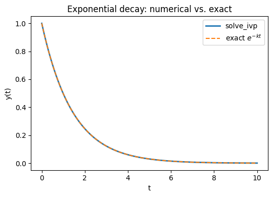
Example: Minimal scalar example – exponential decay

First for a very simple dynamic scalar model we can solve an ODE like:

\[\displaystyle\frac{dy}{dt}=-k\,y,\;y(0)=1\]

using scipy’s integrate package and compare the accuracy with the analytical solution:

import numpy as np
import matplotlib.pyplot as plt
from math import exp
from scipy.integrate import solve_ivp

# --- everything up to this point is exactly what you already have ---
k = 0.7
decay = lambda t, y: -k * y
sol = solve_ivp(decay, t_span=[0, 10], y0=[1.0], rtol=1e-9, atol=1e-12)

# Analytical solution on the same time grid
t_exact = sol.t
y_exact = np.exp(-k * t_exact)

# Plot results
plt.figure(figsize=(5.5, 4))
plt.plot(sol.t, sol.y[0], label='solve_ivp', lw=2)
plt.plot(t_exact, y_exact, '--', label='exact $e^{-kt}$')
plt.xlabel('t')
plt.ylabel('y(t)')
plt.title('Exponential decay: numerical vs. exact')
plt.legend()
plt.tight_layout()
plt.show()

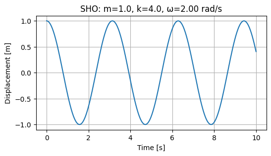
Example: Simple harmonic oscillator with interactive controls

The simple harmonic oscillator (SHO) is a classic example of a dynamic system that can be described by a second-order ordinary differential equation (ODE). The SHO is characterized by its oscillatory motion, which can be described by the equation:

\[ \frac{d^2 y}{dt^2} + \omega^2 y = 0 \]

where \(y\) is the displacement from the equilibrium position, \(\omega\) is the angular frequency, and \(t\) is time. Integrators in standard libraries are always written for first-order systems, so we need to convert this second-order ODE into a system of first-order ODEs. We can always convert the second-order ODE into a system of first-order ODEs using the variable substitution “trick” (cf. Strogatz (2015) or similar textbooks): let \(y = y_1\) and \(y_2 = \frac{dy_1}{dt}\). This yields:

\[ \frac{dy_1}{dt} = y_2 \]

\[ \frac{dy_2 }{dt} = -\omega^2 y_1 \]

or in vector form:

\[\begin{split} \frac{d \mathbf{y} }{dt} = \; \begin{bmatrix} y_2\\ -\omega^2 y_1 \end{bmatrix} \;\end{split}\]

This reduction allows us to apply standard numerical integrators for first-order systems. The SHO can then be solved using numerical methods such as the Runge-Kutta method or the Verlet method. In this example, we will use the scipy.integrate.solve_ivp function to solve the SHO equation and visualize the results.

import numpy as np
import matplotlib.pyplot as plt
from ipywidgets import interact
from scipy.integrate import solve_ivp

def simulate(m=1.0, k=4.0, x0=1.0, v0=0.0, t_end=10.0):
    omega = np.sqrt(k/m)
    def sho(t, y):       # y = [y_1, y_2]
        return [y[1],  # dy_1/dt = y_2
                -omega**2 * y[0]  # dy_2/dt = -ω² y_1
                ]

    sol = solve_ivp(sho, [0, t_end], [x0, v0], max_step=0.05)
    t, x = sol.t, sol.y[0]

    plt.figure(figsize=(6, 3))
    plt.plot(t, x)
    plt.xlabel('Time [s]')
    plt.ylabel('Displacement [m]')
    plt.title(f'SHO: m={m}, k={k}, ω={omega:.2f} rad/s')
    plt.grid(True)
    plt.show()

simulate(m=1.0, k=4.0, x0=1.0, v0=0.0, t_end=10.0)

interact(simulate,
         m=(0.5, 5.0, 0.5),
         k=(1.0, 10.0, 0.5),
         x0=(-2.0, 2.0, 0.2),
         v0=(-2.0, 2.0, 0.2),
         t_end=(2.0, 20.0, 1.0));

2.2 Linear vs. non-linear

	Linear	Non-linear
Abstraction	\(A\,\mathbf{x}= \mathbf{b}\)	\(\mathbf{f}(\mathbf{x}) = \mathbf{0}\)
Typical mathematized examples	\(x_1 + x_2 = 5^2\), \(\frac{d^2y}{dx^2} = k y\)	\(x_1^2 + x_2^2 = 5^2\), \(\frac{dy}{dx} = k y^2\)
Examples in nature	Mass–spring system at small deflection	Duffing oscillator, orbital dynamics

Linearity is an important concept in modelling, linear models are highly desirable because they are easier to analyse and solve. Linear methods are highly scalable to millions of variables and a great effort is made to find linear model representations or to linearize inherently non-linear natural processes. In contrast, non-linear models involve non-linear relationships between variables, making them more complex and often harder to solve.

Definition: Let \(\mathcal{X}\) be a vector space and \(\mathcal{F} : \mathcal{X}\to\mathcal{X}\) a mapping that represents the model (algebraic or differential). \(\mathcal{F}\) is linear iff it satisfies superposition for all \( \mathbf{x},\mathbf{y}\in\mathcal{X}\) and \( \alpha\in\mathbb{R}\):

1. Additivity: \(\mathcal{F}(\mathbf{x}+\mathbf{y}) = \mathcal{F}(\mathbf{x}) + \mathcal{F}(\mathbf{y}) \)

2. Homogeneity: \( \mathcal{F}(\alpha\,\mathbf{x}) = \alpha\,\mathcal{F}(\mathbf{x}) \)

Identifying linearity is partricularly important since linear solvers are far faster and more accurate than non-linear solvers, in the examples below we demonstrate how to write both families in linear standard form.

2.2.1 Multivariable linear static example

Most models you will encounter will likely be written in non-standard form. It’s important to be able to transform the model to standard forms that can be solved with powerful numerical libraries. Consider the following example:

Reaction forces in a satellite-bus support frame (Hibbeler, Engineering Mechanics – Statics, §16-4 “Method of Joints” (numbers differ) • Logan, A First Course in the Finite Element Method, Ex. 2-2)

A triangular support carries a payload mass (m) at node 3. Nodes 1 & 2 are fixed to the bus deck (see figure below). Assuming axial members only (truss), the static equilibrium is

\[\begin{split} \begin{aligned} 8\times10^{5}\,u_1 \;-\;2\times10^{5}\,u_2 \;-\;6\times10^{5}\,u_3 &= 0, \\[4pt] -2\times10^{5}\,u_1 \;+\;8\times10^{5}\,u_2 \;-\;4\times10^{5}\,u_3 &= 0, \\[4pt] -6\times10^{5}\,u_1 \;-\;6\times10^{5}\,u_2 \;+\;1.2\times10^{6}\,u_3 &= -m g. \end{aligned} \end{split}\]

In order to convert this to standard form we must first identify the variables we are trying to solve (in this case clearly \(u_i\)). For this course we will always use \(x_i\) to denote scalar variables while the vector \(\mathbf{x}\) represents contains all the variables of our system \(x_1, x_2, \dots \in \mathbf{x}\). In linear systems these variables always have coefficients \(a_{ij}\) which are contained in the coefficient matrix \(a_{ij} \in \mathbf{A}\). Finally, the constant vector \(b_i \in \mathbf{b}\) must always be moved to the right hand side of the system of equations in the standard form:

\[\begin{split} \mathbf{x} \;=\; \begin{bmatrix} x_1\\ x_2\\ x_3 \end{bmatrix} \;=\; \begin{bmatrix} u_1\\ u_2\\ u_3 \end{bmatrix}, \qquad \mathbf{A} \;=\; \begin{bmatrix} a_{11}&a_{12}&a_{13}\\ a_{21}&a_{22}&a_{23}\\ a_{31}&a_{32}&a_{33} \end{bmatrix}, \qquad \mathbf{b} \;=\; \begin{bmatrix} 0\\ 0\\ -m g \end{bmatrix}, \end{split}\]

with coefficients defined by

\[\begin{split} \begin{aligned} a_{11}= 8{\times}10^{5}, &\; a_{12}= -2{\times}10^{5}, &\; a_{13}= -6{\times}10^{5},\\ a_{21}= -2{\times}10^{5}, &\; a_{22}= 8{\times}10^{5}, &\; a_{23}= -4{\times}10^{5},\\ a_{31}= -6{\times}10^{5}, &\; a_{32}= -6{\times}10^{5}, &\; a_{33}= 1.2{\times}10^{6}. \end{aligned} \end{split}\]

and constants:

\[\begin{split} \begin{aligned} b_{1}= 0,\\ b_{2}= 0,\\ b_{3}= - m g \end{aligned} \end{split}\]

It is always possible to convert linear systems to this standard form, then we are left with the matrix equation:

\[ \boxed{\; \mathbf{A}\,\mathbf{x} = \mathbf{b}\;} . \]

which can be solved easily using a standard linear algebra solver such as numpy:

import numpy as np
from scipy.linalg import solve
A = np.array([[ 8e5, -2e5, -6e5],
              [-2e5,  8e5, -4e5],
              [-6e5, -6e5,  1.2e6]])
m, g = 50.0, 9.81
b = np.array([0, 0, -m*g])
X = solve(A, b)           # solution for x_i
X

array([-0.002289 , -0.0017985, -0.0024525])

Linear algebra solvers are typically very fast and efficient, even for large systems with millions of variables. They are based on matrix factorization methods such as LU decomposition, which allow for efficient solution of linear systems. By contranst non-linear systems cannot be solved with linear algebra solvers, but rather require iterative methods such as Newton’s method or fixed-point iteration such as those introduced earlier and wrapped into scipy.optimize.fsolve or scipy.optimize.root.

2.2.2 Multivariable non-linear static example

While every linear system can be reduced to the matrix form \(\mathbf{A}\mathbf{x}=\mathbf{b}\), non-linear static problems lead to residual equations \(\mathbf{F}(\mathbf{x})=\mathbf{0}\). We must therefore define a vector function \(\mathbf{F}\) instead of a coefficient matrix.

Example: Steady-state heat balance of two radiating CubeSat faces

Consider the steady-state heat balance of two radiating CubeSat faces (Gilmore, Spacecraft Thermal Control Handbook, Ch. 5).

A face receives constant absorbed power \(q_{\text{in},i}\), radiates to deep space (\(T_\text{space}\simeq3\,\)K) and conducts to its neighbour:

\[\begin{split} \begin{aligned} 0 &= q_{\text{in},1} -\varepsilon\sigma A\!\left(T_{1}^{4}-T_{\text{space}}^{4}\right) -G\,(T_{1}-T_{2}), \\[6pt] 0 &= q_{\text{in},2} -\varepsilon\sigma A\!\left(T_{2}^{4}-T_{\text{space}}^{4}\right) +G\,(T_{1}-T_{2}). \end{aligned} \end{split}\]

Identify variables and build the standard non-linear form

• Variables \(\mathbf{x}=\begin{bmatrix}x_1\\x_2\end{bmatrix} =\begin{bmatrix}T_1\\T_2\end{bmatrix}\)

• Residual vector \(\mathbf{F}(\mathbf{x}) =\begin{bmatrix}F_1(\mathbf{x})\\F_2(\mathbf{x})\end{bmatrix}\) with

\[\begin{split} \begin{aligned} F_1(\mathbf{x}) &= q_{\text{in},1} -\varepsilon\sigma A\bigl(x_{1}^{4}-T_{\text{space}}^{4}\bigr) -G\,(x_{1}-x_{2}),\\[4pt] F_2(\mathbf{x}) &= q_{\text{in},2} -\varepsilon\sigma A\bigl(x_{2}^{4}-T_{\text{space}}^{4}\bigr) +G\,(x_{1}-x_{2}). \end{aligned} \end{split}\]

Standard form

\[ \boxed{\; \mathbf{F}(\mathbf{x}) = \mathbf{0}\;} \qquad\Longrightarrow\qquad \text{solve for }\mathbf{x}. \]

This has to be solved with the more expensive scipy.optimize.fsolve family of solvers as we had before:

import numpy as np
from scipy.optimize import fsolve

# physical parameters
eps   = 0.8                      # emissivity
sigma = 5.670374e-8              # Stefan–Boltzmann, W m⁻² K⁻⁴
A     = 0.04                     # 10 cm × 10 cm face, m²
G     = 0.5                      # conductive coupling, W K⁻¹
Tsp   = 3.0                      # deep-space sink temperature, K
qin1, qin2 = 6.0, 2.0            # absorbed power, W

def F(X):
    x1, x2 = X
    F1 = qin1 - eps*sigma*A*(x1**4 - Tsp**4) - G*(x1 - x2)
    F2 = qin2 - eps*sigma*A*(x2**4 - Tsp**4) + G*(x1 - x2)
    return [F1, F2]

T_guess = [300.0, 290.0]         # initial guess, K
T1, T2  = fsolve(F, T_guess)
print(f"T1 = {T1:.1f} K,   T2 = {T2:.1f} K")

T1 = 218.5 K,   T2 = 214.8 K

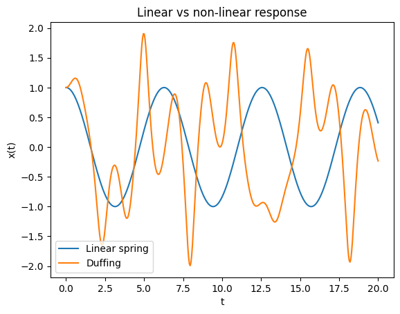
Example: Linear vs non-linear response of a spring

Below we demonstrate the difference between linear and non-linear response of a spring system. The linear spring is described by Hooke’s law, while the Duffing oscillator is a non-linear system that exhibits more complex behavior. The Duffing oscillator is a well-known example of a non-linear system that can exhibit chaotic behavior under certain conditions. The linear spring is described by the equation (F = kx), where (F) is the force, (k) is the spring constant, and (x) is the displacement from the equilibrium position. The Duffing oscillator is described by the equation:

\[\frac{d^2x}{dt^2} + \delta \frac{dx}{ dt} + \alpha x + \beta x^3 = \gamma \cos(\omega t)\]

where \(\delta\) is the damping coefficient, \(\alpha\) and \(\beta\) are the linear and non-linear stiffness coefficients, \(\gamma\) is the amplitude of the driving force, and \(\omega\) is the frequency of the driving force.

The example below uses scipy.integrate.solve_ivp to solve both systems and plot their responses over time. The linear spring will exhibit simple harmonic motion, while the Duffing oscillator will show more complex behavior, especially for larger driving forces or non-linear stiffness coefficients.

import numpy as np
import matplotlib.pyplot as plt
from scipy.integrate import solve_ivp

def linear_spring(t, y, k=1.0, m=1.0):
    x, v = y
    return [v, -k/m * x]

def duffing(t, y, alpha=1.0, beta=5.0, delta=0.02, gamma=8.0, omega=1.2):
    x, v = y
    return [v, -delta*v - alpha*x - beta*x**3 + gamma*np.cos(omega*t)]

sol_lin = solve_ivp(linear_spring, [0, 20], [1, 0], max_step=0.05)
sol_non = solve_ivp(duffing,       [0, 20], [1, 0], max_step=0.05)

plt.plot(sol_lin.t, sol_lin.y[0], label="Linear spring")
plt.plot(sol_non.t, sol_non.y[0], label="Duffing")
plt.xlabel("t"); plt.ylabel("x(t)")
plt.legend(); plt.title("Linear vs non-linear response");

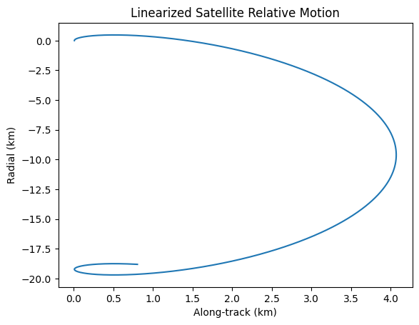
Example: Linearized satellite relative motion

In this example, we will demonstrate the linearized relative motion of a satellite in orbit. The Hill–Clohessy–Wiltshire (HCW) equations describe the relative motion of a chaser satellite about a chief on a circular orbit are a set of linearized equations that describe the relative motion of a satellite in orbit:

\[\begin{split} \begin{aligned} \ddot x & =\;\; 3n^{2}x + 2n\dot y + a_x,\\ \ddot y & = -2n\dot x + a_y,\\ \ddot z & = -n^{2}z + a_z, \end{aligned} \qquad n \;=\;\sqrt{\dfrac{\mu}{a^{3}}}\;, \end{split}\]

where \((x,y,z) \) are radial, along-track, cross-track offsets, \( n \) the mean motion of the chief, \( a_{x,y,z}\) thrust accelerations.

The example below uses scipy.integrate.odeint to solve the hcw equations and plot the relative motion of the satellite.

import numpy as np
from scipy.integrate import odeint
import matplotlib.pyplot as plt

def hcw(y, t, n):
    return [y[3], y[4], y[5], 3*n**2*y[0] + 2*n*y[4], -2*n*y[3], -n**2*y[2]]

n = 0.001  # Orbital rate
y0 = [0.01, 0, 0, 0, 0.001, 0]
t = np.linspace(0, 3600*2, 1000)  # 2 orbits
sol = odeint(hcw, y0, t, args=(n,))
plt.plot(sol[:,0], sol[:,1])
plt.title('Linearized Satellite Relative Motion')
plt.xlabel('Along-track (km)')
plt.ylabel('Radial (km)')
plt.show()

2.3 Coupled vs. uncoupled

Models can be classified based on the degree of interaction between their variables. In uncoupled models, variables or equations evolve independently, allowing for straightforward decomposition and solution. Coupled models, however, feature interactions where changes in one variable directly affect others, often leading to more complex behavior that requires simultaneous solution techniques. This distinction is crucial in computational engineering, as coupling can introduce phenomena like resonance or instability, which are observable through changes in system eigenvalues (e.g., eigenvalue splitting when weak coupling is added to an otherwise uncoupled system).

	Uncoupled	Coupled
Abstraction	\(\mathbf{f}(\mathbf{x}) = \begin{bmatrix} f_1(x_1) \\ f_2(x_2) \\ \vdots \\ f_n(x_n) \end{bmatrix} = \mathbf{0}\) or independent ODEs	\(\mathbf{f}(\mathbf{x}) = \mathbf{0}\) where components of \(\mathbf{f}\) depend on multiple \(x_i\)
Typical mathematized examples	\(x_1 = 5\), \(x_2 = 3\) (independent equations); \(\frac{dx_1}{dt} = k_1 x_1\), \(\frac{dx_2}{dt} = k_2 x_2\) (independent ODEs)	\(x_1 + x_2 = 5\), \(x_1 - x_2 = 3\); \(\frac{dx_1}{dt} = k_1 x_1 + k_2 x_2\), \(\frac{dx_2}{dt} = k_3 x_1 + k_4 x_2\)
Examples in nature	Three orthogonal resistors in parallel on an electrical breadboard (currents independent)	3D attitude dynamics of a spacecraft, where roll, pitch, and yaw angles interact via inertial cross-products

Definition: Let \(\mathcal{X}\) be a vector space and \(\mathcal{F} : \mathcal{X} \to \mathcal{X}\) a mapping representing the model (algebraic or differential). The model is uncoupled if \(\mathcal{F}\) can be decomposed into independent sub-mappings \(\mathcal{F}_i : \mathcal{X}_i \to \mathcal{X}_i\) such that \(\mathcal{F}(\mathbf{x}) = (\mathcal{F}_1(x_1), \mathcal{F}_2(x_2), \dots, \mathcal{F}_n(x_n))\) where the \(\mathcal{X}_i\) are disjoint subspaces. Otherwise, it is coupled, meaning at least one component of \(\mathcal{F}\) depends on variables from multiple subspaces.

(Observe how eigenvalues split when coupling is introduced, e.g., in a mass spring system where adding a cross spring shifts degenerate modes.)

You will learn about coupled vs. uncoupled systems in more detail in Week 3, where we will also discuss the implications of coupling on system stability and dynamics. For now it is important to understand that uncoupled systems can be solved independently, while coupled systems require simultaneous solution techniques, such as matrix methods or iterative solvers.

2.4 Symmetry

Models often exhibit symmetries, which are invariances under certain transformations (e.g., rotations, translations, or time shifts). Recognizing symmetry simplifies computations by reducing degrees of freedom, enabling the use of group theory or conservation laws. In computational engineering, symmetries lead to efficient algorithms, such as modal analysis in structural dynamics or exploiting rotational invariance in orbital mechanics. This will be expanded in Week 3 with connections to conservation laws via Noether’s theorem, which links continuous symmetries to conserved quantities like energy or momentum.

	Symmetric	Asymmetric
Abstraction	Model invariant under group action \(G\), i.e., \(\mathcal{F}(g \cdot \mathbf{x}) = g \cdot \mathcal{F}(\mathbf{x})\) for \(g \in G\)	No such invariance under non-trivial transformations
Typical mathematized examples	Laplace’s equation in a sphere: \(\nabla^2 \phi = 0\) (rotational symmetry); Hamiltonian systems with time-independence (energy conservation)	\(\frac{dx}{dt} = x + t\) (breaks time-translation symmetry); Non-uniform truss with irregular loading
Examples in nature	Planetary orbits under central gravity (rotational symmetry)	Asymmetric airfoil in aerodynamics (directional lift dependence)

Definition: Let \(\mathcal{X}\) be a vector space, \(G\) a symmetry group (e.g., rotations \(SO(3)\) or translations \(\mathbb{R}^3\)), and \(\cdot : G \times \mathcal{X} \to \mathcal{X}\) a group action. A model mapping \(\mathcal{F} : \mathcal{X} \to \mathcal{X}\) is symmetric under \(G\) if \(\mathcal{F}(g \cdot \mathbf{x}) = g \cdot \mathcal{F}(\mathbf{x})\) for all \(g \in G\) and \(\mathbf{x} \in \mathcal{X}\). It is asymmetric if no non-trivial symmetry group exists.

Identifying symmetries in models is crucial for simplifying computations and understanding the underlying physics. A rule of thumb that allows to be easily identified in a model is that if the indices of the variables can be interchanged then the variables are symmetric. For example, in:

\[ f(x_1, x_2, x_3) = \sum_{i=1}^3 x_i^2 + \prod_{i=1}^3 sin(x_i) = x_1^2 + x_2^2 + x_3^2 + \sin(x_1) \sin(x_2) \sin(x_3) \]

the variables \(x_i\) can be interchanged without changing the form of function, indicating symmetry. Natural symmetries can also lead to conservation laws, which are powerful tools in both analytical and numerical methods. In computational engineering, exploiting symmetries can significantly reduce the complexity of simulations, leading to faster and more efficient algorithms. You will learn more about symmetries in Week 7 and 9 where we exploit symmetries to drastically reduce the cost of computational models.

Using SymPy to spot simple symmetries

Below is a minimal utility that checks whether a symbolic expression stays unchanged under

1. Permutations of a list of variables (useful for detecting interchange symmetry \(x_i \leftrightarrow x_j\)), and

2. User-supplied transformations (e.g. planar rotations).

import sympy as sp
from itertools import permutations

# 1.  Generic invariance tester
def is_invariant(expr, transform):
    """
    Return True if expr(variables) == expr after applying `transform`,
    where `transform` is a dict {old_symbol: new_symbol_or_expr}.
    """
    transformed = expr.xreplace(transform)
    return sp.simplify(expr - transformed) == 0

# 2.  Convenience wrapper for permutation symmetry
def permutation_symmetries(expr, variables):
    """
    List all permutations of `variables` that leave `expr` unchanged.
    """
    invariants = []
    for p in permutations(variables):
        mapping = dict(zip(variables, p))
        if is_invariant(expr, mapping):
            invariants.append(p)
    return invariants

Example: permutation symmetry in f(x1,x2,x3)

Below we expect all 6 permutations in the full S₃ symmetry group to be found, since the expression is symmetric in all three variables.

\[ f(x_1, x_2, x_3) = x_1^2 + x_2^2 + x_3^2 + \sin(x_1) \sin(x_2) \sin(x_3)\]

This is a simple example of how to use the permutation_symmetries function to find symmetries in a symbolic expression.

x1, x2, x3 = sp.symbols('x1 x2 x3')
expr = (x1**2 + x2**2 + x3**2) + sp.sin(x1)*sp.sin(x2)*sp.sin(x3)

perms = permutation_symmetries(expr, (x1, x2, x3))
print("Permutations that keep the expression unchanged:")
for p in perms:
    print("  ", p)

Permutations that keep the expression unchanged:
   (x1, x2, x3)
   (x1, x3, x2)
   (x2, x1, x3)
   (x2, x3, x1)
   (x3, x1, x2)
   (x3, x2, x1)

Example: rotational symmetry \(f(r, \theta)\) in 2-D

The function below depends only on \(r\) and not on the angle \(\theta\) despite this being declared as a variable in the mode:

\[ r = \sqrt{x^2 + y^2} \]

\[f(r, \theta) = e^{-r}\]

This is a simple example of how to use the is_invariant function to check for rotational symmetry in a symbolic expression. The function checks whether the expression remains unchanged under the specified transformation, which in this case is a rotation in 2D space.

x, y, θ = sp.symbols('x y θ')
r = sp.sqrt(x**2 + y**2)
f_r = sp.exp(-r)

rotation = {x:  x*sp.cos(θ) - y*sp.sin(θ),
            y:  x*sp.sin(θ) + y*sp.cos(θ)}

print("Rotationally invariant?", is_invariant(f_r, rotation))

Rotationally invariant? True

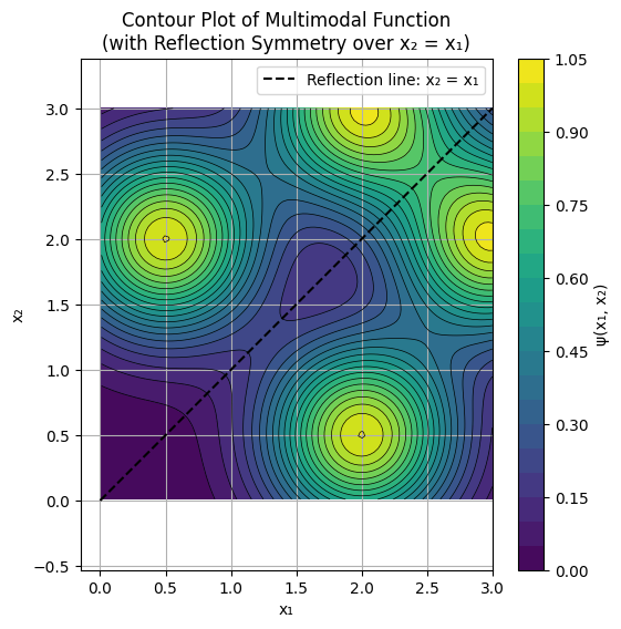
Example: Demonstration of numerical use of symmetry with a multimodal potential function

It’s import to not lose sight of the inherent geometric meaning of symmetry, for example the potential function:

\[\psi(x_1, x_2) = e^{ -\frac{(x_1 - 3)^2 + (x_2 - 2)^2}{0.5} } + e^{ -\frac{(x_1 - 2)^2 + (x_2 - 3)^2}{0.5} } + e^{ -\frac{(x_1 - 0.5)^2 + (x_2 - 2)^2}{0.5} } + e^{ -\frac{(x_1 - 2)^2 + (x_2 - 0.5)^2}{0.5} }, \]

is plotted below, notice the reflection line \(x_2 = x_1\). The practical implications of this are myriad. For example:

1. If we have an expensive function, there is no need to compute anything in the domain above the \(x_2 = x_1\) line since we could simply retrieve those function values for \(\psi(x_1, x_2)\) by reflecting the input \(\psi(x_2, x_1) = \psi(x_1, x_2)\).

2. In optimization, we can add the constraint \(x_2 < x_1 \forall ~~\mathbf{x} \in \mathcal{X}\) since any minima found below the \(x_2 = x_1\) also automitically retrieve the objective function value by again simply reflecting the variables, so we never learn any new information by exploring above the \(x_2 = x_1\) line.

In higher dimensions these concepts are even more valuable, saving us extreme computational time in factorial order \(\mathcal{O}(d!)\).

import numpy as np
import matplotlib.pyplot as plt

# Define grid: first quadrant, x1 > 0, x2 > 0
x = np.linspace(0.01, 3, 100)  # Fine grid; try 20 for coarse to see discretization effects
y = np.linspace(0.01, 3, 100)
X1, X2 = np.meshgrid(x, y)

# Multimodal function (sum of Gaussians, symmetric across x2 = x1)
psi = (np.exp(- ((X1 - 3)**2 + (X2 - 2)**2) / 0.5) +
       np.exp(- ((X1 - 2)**2 + (X2 - 3)**2) / 0.5) +
       np.exp(- ((X1 - 0.5)**2 + (X2 - 2)**2) / 0.5) +
       np.exp(- ((X1 - 2)**2 + (X2 - 0.5)**2) / 0.5)
       )

# Contour plot to visualize multimodal structure and symmetry
plt.figure(figsize=(6, 6))
plt.contourf(X1, X2, psi, levels=20, cmap='viridis')  # Filled contours
plt.colorbar(label='ψ(x₁, x₂)')
plt.contour(X1, X2, psi, levels=20, colors='black', linewidths=0.5)  # Outline contours

# Draw the reflection line x2 = x1
plt.plot([0, 3], [0, 3], 'k--', label='Reflection line: x₂ = x₁')

plt.xlabel('x₁')
plt.ylabel('x₂')
plt.title('Contour Plot of Multimodal Function\n(with Reflection Symmetry over x₂ = x₁)')
plt.axis('equal')  # Preserve aspect ratio for accurate symmetry visualization
plt.legend()
plt.grid(True)
plt.show()

Conclusions

In this chapter we have introduced a basic classification scheme for models based on four key properties: static vs. dynamic, linear vs. non-linear, coupled vs. uncoupled, and symmetric vs. asymmetric. We learned how to solve basic simulation problems using Python libraries such as numpy and scipy.

Understanding these properties is crucial for selecting appropriate numerical methods and solvers, as they directly impact the complexity and computational cost of solving the models. In the next chapter we will discuss the concept of degrees of freedom and how to count them in models while expanding our toolset of modeling techniques.

Further reading

• The scipy user guide as a starting point for exploring common numerical methods: https://docs.scipy.org/doc/scipy/tutorial/index.html#user-guide

• Historical reference in the development of Statics: Jordan of Nemore, Scientia de Ponderibus, 1565

In the next section we will discuss degrees of freedom and how to count them in models.