Chapter 7: Convex and Linear Optimization

Chapter 7: Convex and Linear Optimization#

7.1 Optimization in general#

Optimization is a fundamental tool in engineering, used to find the “best” solution among many possibilities—such as minimizing fuel consumption in spacecraft trajectories or maximizing structural efficiency under constraints. Unlike the algebraic systems in Chapter 4 (where we solved for exact equality, like $\mathbf{F}(\mathbf{x}) = \mathbf{0}$), optimization problems are typically underdetermined: there are more variables (degrees of freedom) than equations, leading to infinitely many feasible solutions. We seek the one that extremizes (minimizes or maximizes) an objective function while satisfying constraints.

7.1.1 Formal Statement of the General Optimization Problem#

A general optimization problem can be stated as:

\[\begin{split} \begin{align*} \min_{\mathbf{x}} \quad & f(\mathbf{x}) \\ \text{subject to} \quad & \mathbf{g}(\mathbf{x}) \leq \mathbf{0}, \\ & \mathbf{h}(\mathbf{x}) = \mathbf{0}, \\ & \mathbf{x} \in \mathcal{X}, \end{align*} \end{split}\]

where:

$\mathbf{x} \in \mathbb{R}^n$ is the vector of decision variables (e.g., design parameters or control inputs).
$f: \mathbb{R}^n \to \mathbb{R}$ is the scalar objective function to minimize (for maximization, use $\max -f(\mathbf{x})$).
$\mathbf{g}: \mathbb{R}^n \to \mathbb{R}^m$ are inequality constraints (e.g., resource limits like $x_1 + x_2 \leq 10$).
$\mathbf{h}: \mathbb{R}^n \to \mathbb{R}^p$ are equality constraints (e.g., conservation laws like $x_1 - x_2 = 0$).
$\mathcal{X}$ is the feasible domain (e.g., bounds like $\mathbf{x}_L \leq \mathbf{x} \leq \mathbf{x}_U$ or integer requirements).

Here, $n > m + p$ typically holds, making the problem underdetermined, i.e. multiple $\mathbf{x}$ satisfy the constraints, and we optimize over them. The feasible set is $\{\mathbf{x} \in \mathcal{X} \mid \mathbf{g}(\mathbf{x}) \leq \mathbf{0}, \mathbf{h}(\mathbf{x}) = \mathbf{0}\}$, and the goal is to find a local or global minimum within it. A standard optimization problem is usually stated as minimization; maximization can be handled by minimizing the negative of the objective, i.e. $\min_{\mathbf{x}} f(\mathbf{x}) = \max_{ \mathbf{x}}- f(\mathbf{x})$.

In general, numerical optimization methods are based on sampling information of the objective function $f$ by iteratively sampling the function at successive points $\mathbf{x}$. For example, the crudest approach is brute force search, which samples $f$ at a grid of points in $\mathcal{X}$ and picks the best. More sophisticated methods use gradient or Hessian information to guide the search more efficiently (covered in later sections).

7.1.2 Brute Force Search: A Simple Visual Demonstration in Python#

Bruth force search in the context of optimization can refer to either attempting all combinations of a combinatorial (or mixed integer) problem or uniform sampling of the domain $\mathcal{X}$ in the case where $f$ is continuous. A simple implementation is demonstrated in the following example:

Example: Brute force search

For the simplest case, consider a 1D unconstrained problem: minimize $f(x) = x^2 + \sin(2\pi x)$ over $x \in [-2, 2]$. This can be naively “optimized” by evaluating on a grid and sorting (like argmin), but real methods are more efficient. Here’s a Python demonstration plotting the function and finding its minimum using basic grid search:

import numpy as np
import matplotlib.pyplot as plt

# Define the objective function
def f(x):
    return x**2 + np.sin(2 * np.pi * x)

# Generate 60 sampling points and evaluate f(x) at every point:
x = np.linspace(-2, 2, 60)
y = f(x)
y = np.array(y)
x = np.array(x)

# Simple grid search for minimum (argmin)
min_idx = np.argmin(y)
x_min = x[min_idx]
y_min = y[min_idx]

# Plot
plt.figure(figsize=(8, 4))
plt.plot(x, y, label='$f(x) = x^2 + \sin(2\pi x)$', alpha=0.5)
plt.scatter(x, y, marker='o', color='gray', alpha=0.7, label=f'Points sampled with brute force search')
plt.scatter(x_min, y_min, marker='X', color='red', label=f'Minimum found at x={x_min:.2f}, f(x)={y_min:.2f}')
plt.xlabel('x')
plt.ylabel('f(x)')
plt.legend()
plt.grid(True)
plt.show()

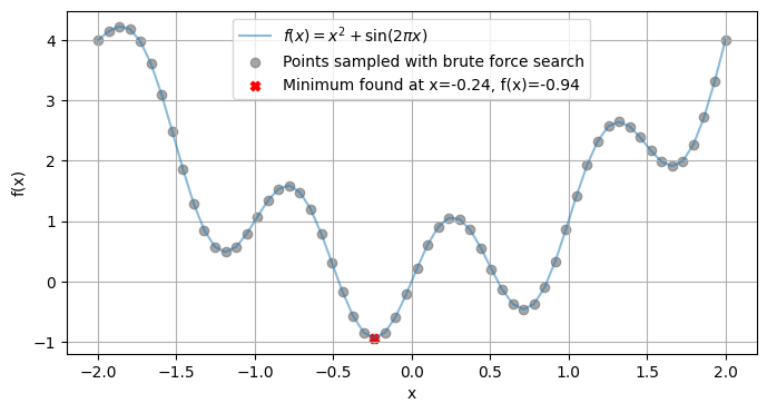
../_images/a82121168642ba3d5d577f1d43dab4bd872c04be101d74f12607f5339f0a0253.png

This grid approach mimics sorting for argmin in 1D but scales poorly to higher dimensions, real algorithms (like those in later sections) use gradients or search strategies.

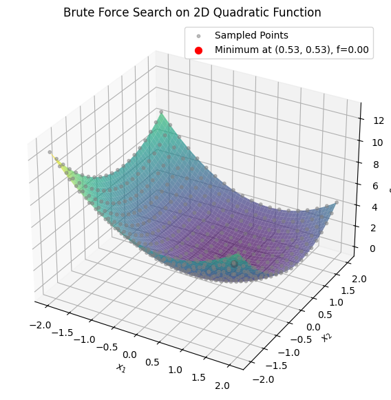
Example: Brute Force on a 2D Quadratic Function

To extend brute force search to higher dimensions, consider a 2D unconstrained problem: minimize $f(x_1, x_2) = (x_1 - 0.5)^2 + (x_2 - 0.5)^2$ over $x_1, x_2 \in [-2, 2]$. This is a quadratic function with a minimum at (0.5, 0.5). We’ll use a meshgrid to sample points, evaluate the function, and find the minimum via argmin on the flattened array. Here’s the Python code for sampling, finding the minimum, and visualizing with a 3D surface plot:

import numpy as np
import matplotlib.pyplot as plt
from mpl_toolkits.mplot3d import Axes3D

# Define the objective function
def f(x1, x2):
    return (x1 - 0.5)**2 + (x2 - 0.5)**2

# Generate a 20x20 grid for brute force sampling (fewer points for illustration)
x1 = np.linspace(-2, 2, 20)
x2 = np.linspace(-2, 2, 20)
X1, X2 = np.meshgrid(x1, x2)
Z = f(X1, X2)

# Find the minimum on the grid
min_idx = np.argmin(Z)
min_row, min_col = np.unravel_index(min_idx, Z.shape)
x1_min = X1[min_row, min_col]
x2_min = X2[min_row, min_col]
z_min = Z[min_row, min_col]

# For denser plot surface (100x100)
x1_dense = np.linspace(-2, 2, 100)
x2_dense = np.linspace(-2, 2, 100)
X1_dense, X2_dense = np.meshgrid(x1_dense, x2_dense)
Z_dense = f(X1_dense, X2_dense)

# Plot 3D surface
fig = plt.figure(figsize=(10, 7))
ax = fig.add_subplot(111, projection='3d')
ax.plot_surface(X1_dense, X2_dense, Z_dense, cmap='viridis', alpha=0.7)
ax.scatter(X1.flatten(), X2.flatten(), Z.flatten(), color='gray', alpha=0.5, s=10, label='Sampled Points')
ax.scatter(x1_min, x2_min, z_min, color='red', s=50, label=f'Minimum at ({x1_min:.2f}, {x2_min:.2f}), f={z_min:.2f}')
ax.set_xlabel('$x_1$')
ax.set_ylabel('$x_2$')
ax.set_zlabel('$f(x_1, x_2)$')
ax.set_title('Brute Force Search on 2D Quadratic Function')
ax.legend()
plt.show()

../_images/25e08b710cf7ec50af24d4fc5984e2506df6f2c98abe869fc40df82a13654efc.png

In Chapter 4, we solved nonlinear algebraic systems $\mathbf{F}(\mathbf{x}) = \mathbf{0}$ using Gauss-Newton, which iteratively minimizes the residual $\|\mathbf{F}(\mathbf{x})\|^2$ via linear approximations. This is a special case of optimization: an unconstrained nonlinear least-squares problem. For example, Gauss-Newton uses Jacobian-based updates, akin to gradient descent (covered in 7.7), but tailored for residuals. We’ll generalize this in linear least-squares (7.6) and nonlinear variants next week.

7.2 Classification of common optimization problems#

Optimization problems can be classified based on several key characteristics, such as the nature of the objective function $f$ (linear vs. nonlinear), the types of constraints ($\mathbf{g}$ and $\mathbf{h}$), the presence of integer variables, and whether derivatives are available or needed. This classification helps in selecting appropriate algorithms, as different types have varying computational complexities and guarantees (e.g., convexity often ensures global optimality for local solvers).

Below is a table summarizing common categories and subcategories. Note that many problems can overlap (e.g., an LP is also convex), and this is not exhaustive but covers the most relevant types for computational engineering. We’ll explore linear/convex types in this chapter, nonlinear in Chapter

Category	Subcategory	Description	Examples/Notes
Convex Optimization	Linear Programming (LP)	Objective and constraints are linear; feasible region is a polytope. Guarantees global optimum.	Resource allocation, e.g., minimizing cost subject to linear inequalities. Solved with simplex or interior-point methods.
	Quadratic Programming (QP)	Quadratic objective with linear constraints; convex if the Hessian is positive semi-definite.	Portfolio optimization, least-squares with bounds.
	Semidefinite Programming (SDP)	Involves optimizing over positive semidefinite matrices; generalizes LP/QP.	Control theory, eigenvalue optimization.
Nonlinear Programming (NLP)	Convex NLP	Nonlinear objective/constraints, but the problem remains convex (e.g., via convex functions).	Logistic regression, some fluid dynamics models.
	Nonconvex NLP	Nonlinear and nonconvex; may have multiple local optima.	Neural network training, trajectory optimization in space engineering.
Integer Programming	Mixed-Integer Linear Programming (MILP)	LP with some variables restricted to integers.	Scheduling, network design with discrete choices. Branch-and-bound methods.
	Mixed-Integer Nonlinear Programming (MINLP)	NLP with integer variables; combines discrete and continuous optimization.	Process design in chemical engineering, e.g., selecting equipment types.
Global Optimization (GO)	Deterministic GO	Guarantees global optimum for nonconvex problems using exhaustive methods.	Branch-and-bound for global NLP, spatial partitioning. Computationally expensive.
	Stochastic GO	Uses randomness to explore; no global guarantee but practical for high dimensions.	Genetic algorithms, simulated annealing for black-box problems.
Derivative-Free Optimization (DFO)	Model-Based DFO	Builds surrogate models without derivatives.	Bayesian optimization, useful when gradients are unavailable or noisy.
	Direct Search DFO	Pattern or grid-based searches, no derivatives needed.	Nelder-Mead simplex, for simulation-based optimization in engineering.
Other Specialized Types	Stochastic Programming	Handles uncertainty in parameters (e.g., via expectations or scenarios).	Risk-averse optimization in space mission planning under variable conditions.
	Multi-Objective Optimization (MOO)	Optimizes multiple conflicting objectives; yields Pareto fronts.	Trade-off analysis, e.g., minimizing mass vs. maximizing reliability in spacecraft design.

For more details, refer to textbooks like Convex Optimization by Boyd and Vandenberghe (for convex types) or Nonlinear Programming by Bertsekas (for NLP/MINLP). In practice, libraries like SciPy (e.g., scipy.optimize) handle many of these, with specialized solvers like Gurobi or CVXPY for LP/MILP.

7.3 Convexity#

Convexity is a very important concept in optimization because it guarantees that any local minimum is also a global minimum, allowing efficient algorithms to find optimal solutions without getting stuck in suboptimal points. Many real-world engineering problems (e.g., least-squares fitting or linear resource allocation) are convex or can be reformulated as such. Nonconvex problems, however, may require more advanced techniques like those in Chapters 8–9. Formal Definition A function $f: \mathbb{R}^n \to \mathbb{R}$ is convex if, for any $\mathbf{x}, \mathbf{y}$ in its domain and any $\lambda \in [0, 1]$, the following inequality holds: $$f(\lambda \mathbf{x} + (1 - \lambda) \mathbf{y}) \leq \lambda f(\mathbf{x}) + (1 - \lambda) f(\mathbf{y}).$$ Geometrically, this means the line segment connecting any two points on the graph of $f$ lies above or on the graph itself. A set $\mathcal{X}$ is convex if the line segment between any two points in $\mathcal{X}$ remains in $\mathcal{X}$. An optimization problem is convex if the objective $f$ is convex, the inequality constraints $\mathbf{g}$ define convex sets (i.e., $\mathbf{g}$ are convex functions), and equality constraints $\mathbf{h}$ are affine (linear plus constant). If the Hessian $\nabla^2 f$ is positive semi-definite everywhere, $f$ is convex (for twice-differentiable functions).

Example: Python Demonstration of Convexity

To illustrate, we’ll use an interactive widget (via ipywidgets) to visualize the definition. Select two points $a$ and $b$ ($a < b$) on the domain $[-2, 2]$. The plot shows:

Left subplot: A convex function $f(x) = x^2$. The line segment stays above the curve. Right subplot: A nonconvex function $f(x) = x^4 - 3x^2$ (with a “bump” or local maximum at $x=0$). The line segment can intersect or go below the curve, violating convexity.

Adjust the sliders to see how the line behaves for different points.

import numpy as np
import matplotlib.pyplot as plt
from ipywidgets import interact, FloatSlider

# Define the functions
def convex_func(x):
    return x**2

def nonconvex_func(x):
    return x**4 - 3 * x**2

# Interactive plotting function
def plot_convexity(a=-1.0, b=1.0):
    if a >= b:
        print("Please set a < b.")
        return

    x = np.linspace(-2, 2, 1000)

    # Subset for line segment (between a and b)
    mask = (x >= a) & (x <= b)
    x_segment = x[mask]

    # Convex function
    y_convex = convex_func(x)
    y_line_convex = convex_func(a) + (x_segment - a) * (convex_func(b) - convex_func(a)) / (b - a)

    # Nonconvex function
    y_nonconvex = nonconvex_func(x)
    y_line_nonconvex = nonconvex_func(a) + (x_segment - a) * (nonconvex_func(b) - nonconvex_func(a)) / (b - a)

    # Create subplots
    fig, axs = plt.subplots(1, 2, figsize=(12, 5))

    # Convex plot
    axs[0].plot(x, y_convex, label='$f(x) = x^2$ (Convex)', color='blue')
    axs[0].plot(x_segment, y_line_convex, label='Line segment', color='red', linestyle='--')
    axs[0].scatter([a, b], [convex_func(a), convex_func(b)], color='green', zorder=5)
    axs[0].set_title('Convex Function')
    axs[0].set_xlabel('x')
    axs[0].set_ylabel('f(x)')
    axs[0].legend()
    axs[0].grid(True)

    # Nonconvex plot
    axs[1].plot(x, y_nonconvex, label='$f(x) = x^4 - 3x^2$ (Nonconvex)', color='blue')
    axs[1].plot(x_segment, y_line_nonconvex, label='Line segment', color='red', linestyle='--')
    axs[1].scatter([a, b], [nonconvex_func(a), nonconvex_func(b)], color='green', zorder=5)
    axs[1].set_title('Nonconvex Function')
    axs[1].set_xlabel('x')
    axs[1].set_ylabel('f(x)')
    axs[1].legend()
    axs[1].grid(True)

    plt.tight_layout()
    plt.show()

# Create sliders
a_slider = FloatSlider(min=-2, max=2, step=0.1, value=-1.5, description='a:')
b_slider = FloatSlider(min=-2, max=2, step=0.1, value=1.5, description='b:')

interact(plot_convexity, a=a_slider, b=b_slider);

7.4 Linear programming (LP)#

Linear Programming (LP) is a subset of convex optimization where both the objective function and constraints are linear. It is widely used in engineering for problems like resource allocation, scheduling, and trajectory planning in space systems (e.g., optimizing fuel use under linear constraints on thrust and velocity).

Definition: A Linear Programming (LP) problem in standard form is:

\[\begin{split}\begin{align*} \min_{\mathbf{x}} \quad & \mathbf{c}^\top \mathbf{x} \\ \text{subject to} \quad & \mathbf{A} \mathbf{x} = \mathbf{b}, \\ & \mathbf{x} \geq \mathbf{0}, \end{align*}\end{split}\]

where: $\mathbf{x} \in \mathbb{R}^n$ is the vector of non-negative decision variables. $\mathbf{c} \in \mathbb{R}^n$ is the cost vector (objective coefficients). $\mathbf{A} \in \mathbb{R}^{m \times n}$ is the constraint matrix. $\mathbf{b} \in \mathbb{R}^m$ is the right-hand side vector.

Inequality constraints can be converted to this form using slack variables. The feasible region is a convex polytope (intersection of half-spaces), and the optimum occurs at a vertex due to the fundamental theorem of LP. LPs can also be written in canonical form with inequalities: $$\begin{align*} \min_{\mathbf{x}} \quad & \mathbf{c}^\top \mathbf{x} \\ \text{subject to} \quad & \mathbf{A} \mathbf{x} \leq \mathbf{b}, \\ & \mathbf{x} \geq \mathbf{0}. \end{align*}$$ Examples with 2D and 3D Shaded Domains (Convex Polytope) 2D Example Consider maximizing $z = x_1 + x_2$ subject to:

$x_1 \geq 0$, $x_2 \geq 0$, $x_1 + x_2 \leq 2$, $x_1 \leq 1.5$, $x_2 \leq 1$.

The feasible region is a convex polygon. Here’s a Python visualization shading the polytope:

import numpy as np
import matplotlib.pyplot as plt
from matplotlib.patches import Polygon

# Define vertices of the feasible region (convex polytope)
vertices = np.array([[0, 0], [1.5, 0], [1.5, 0.5], [1, 1], [0, 1]])

# Plot the feasible region
fig, ax = plt.subplots(figsize=(6, 6))
poly = Polygon(vertices, closed=True, facecolor='lightblue', edgecolor='blue', alpha=0.5)
ax.add_patch(poly)
ax.plot(vertices[:, 0], vertices[:, 1], 'bo')  # Vertices

# Objective function contours (for illustration)
x1 = np.linspace(0, 2, 100)
x2 = np.linspace(0, 2, 100)
X1, X2 = np.meshgrid(x1, x2)
Z = X1 + X2
ax.contour(X1, X2, Z, levels=10, colors='gray', linestyles='dashed')

ax.set_xlabel('$x_1$')
ax.set_ylabel('$x_2$')
ax.set_title('2D LP Feasible Region (Convex Polytope)')
ax.set_xlim([-0.5, 2])
ax.set_ylim([-0.5, 2])
ax.grid(True)
plt.show()

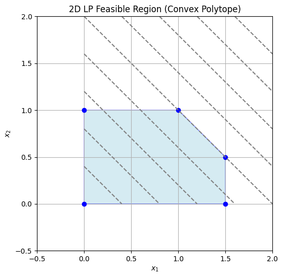
../_images/8accc4f5460b148a0b6b34c36dde7b7bf9ea86ee0d03fd3f10e8ba5efec5d239.png

The optimum is at a vertex, e.g., (1,1) with $z=2$. 3D Example For a 3D LP, maximize $z = x_1 + x_2 + x_3$ subject to:

$x_1, x_2, x_3 \geq 0$, $x_1 + x_2 + x_3 \leq 1$.

The feasible region is a tetrahedron (convex polytope). Visualizing in Python:

import numpy as np
import matplotlib.pyplot as plt
from mpl_toolkits.mplot3d.art3d import Poly3DCollection

# Vertices of the tetrahedron
verts = [
    [[0,0,0], [1,0,0], [0,1,0]],
    [[0,0,0], [1,0,0], [0,0,1]],
    [[0,0,0], [0,1,0], [0,0,1]],
    [[1,0,0], [0,1,0], [0,0,1]]
]

fig = plt.figure(figsize=(8, 8))
ax = fig.add_subplot(111, projection='3d')
ax.add_collection3d(Poly3DCollection(verts, facecolors='lightblue', linewidths=1, edgecolors='blue', alpha=0.5))

ax.scatter([0,1,0,0], [0,0,1,0], [0,0,0,1], color='red', s=50)  # Vertices

ax.set_xlabel('$x_1$')
ax.set_ylabel('$x_2$')
ax.set_zlabel('$x_3$')
ax.set_title('3D LP Feasible Region (Convex Polytope)')
ax.set_xlim([0,1])
ax.set_ylim([0,1])
ax.set_zlim([0,1])
plt.show()

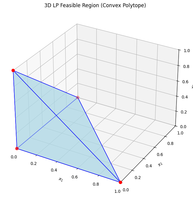
../_images/34590b89935751faaa4afad73637ab90f976987d497343663dd74aa6e8db7964.png

The optimum could be at vertices like (1,0,0) with $z=1$.

7.4.1 Simplex method#

The simplex method, developed by George Dantzig, solves LPs by moving along the edges of the polytope from vertex to vertex, improving the objective at each step. It uses a tableau to represent the system, performing pivot operations to introduce basic variables while maintaining feasibility. Basics:

Start at a basic feasible solution (e.g., origin).
Choose a pivot column (most negative reduced cost for minimization).
Pivot row: Minimum ratio test to maintain non-negativity.
Repeat until no improving direction.

A step by step explanation requires understanding of a tableau and a basic feasible solution.:

Definition:

Tableau:A tabular representation of the LP in standard form, organizing the coefficients of $\mathbf{A}$, $\mathbf{b}$, $\mathbf{c}$, and basic variables. It includes rows for constraints and the objective, with columns for variables (basic and non-basic) and the right-hand side. Pivoting updates the tableau to reflect new basic feasible solutions.

Definition:

Basic Feasible Solution (BFS): A solution where $m$ variables (basic) satisfy the equality constraints $\mathbf{A} \mathbf{x} = \mathbf{b}$, with the remaining $n-m$ variables (non-basic) set to zero. It is feasible if all $\mathbf{x} \geq \mathbf{0}$. BFS correspond to vertices of the polytope.

Visual Step-by-Step Example Using the 2D example: Maximize $z = x_1 + x_2$ (or minimize $-z = -x_1 - x_2$) s.t. $x_1 + x_2 \leq 2$, $x_1 \leq 1.5$, $x_2 \leq 1$, $x_1, x_2 \geq 0$. Introduce slacks $s_1, s_2, s_3 \geq 0$ for inequalities. Initial tableau (standard form, minimize $\mathbf{c}^\top \mathbf{x}$ with $\mathbf{c} = [-1, -1, 0, 0, 0]$):

Basis	$x_1$	$x_2$	$s_1$	$s_2$	$s_3$	RHS
$s_1$	1	1	1	0	0	2
$s_2$	1	0	0	1	0	1.5
$s_3$	0	1	0	0	1	1
$z$	-1	-1	0	0	0	0

Initial BFS: (0,0), $z=0$ (selected point: origin).

Step 1: Pivot column = $x_1$ or $x_2$ (both -1; choose $x_1$). Pivot row = min(2/1, 1.5/1, 1/0=∞) = row 2 (1.5). Pivot, new tableau:

Basis	$x_1$	$x_2$	$s_1$	$s_2$	$s_3$	RHS
$s_1$	0	1	1	-1	0	0.5
$x_1$	1	0	0	1	0	1.5
$s_3$	0	1	0	0	1	1
$z$	0	-1	0	1	0	1.5

New BFS: (1.5, 0), $z=1.5$. Step 2: Pivot column = $x_2$ (-1). Pivot row = min(0.5/1, 1/0=∞, 1/1) = row 1 (0.5). Pivot, new tableau:

Basis	$x_1$	$x_2$	$s_1$	$s_2$	$s_3$	RHS
$x_2$	0	1	1	-1	0	0.5
$x_1$	1	0	-1	2	0	1
$s_3$	0	0	-1	1	1	0.5
$z$	0	0	1	0	0	2

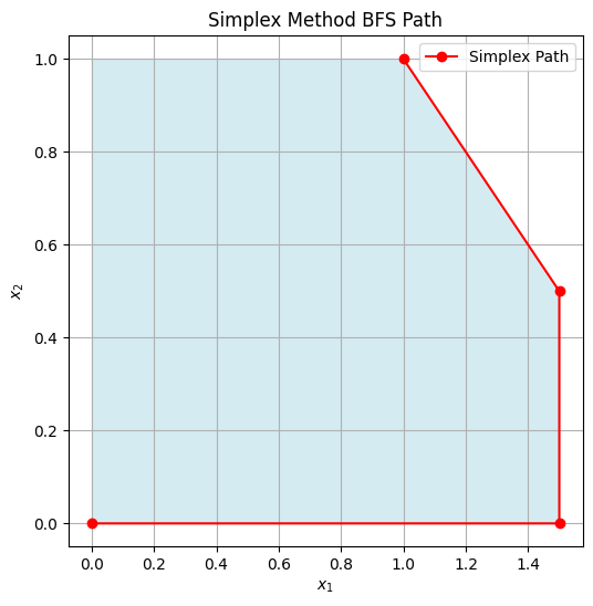
New BFS after proper pivoting, now continue until optimal. (For brevity, steps lead to (1,1) as optimal.) Visual: Points: Start (0,0) → (1.5,0) → (1.5,0.5) → (1,1). Here’s a plot showing BFS points:

import matplotlib.pyplot as plt
import numpy as np
from matplotlib.patches import Polygon

vertices = np.array([[0, 0], [1.5, 0], [1.5, 0.5], [1, 1], [0, 1]])
bfs_points = np.array([[0,0], [1.5,0], [1.5,0.5], [1,1]])  # Example steps

fig, ax = plt.subplots(figsize=(6,6))
poly = Polygon(vertices, facecolor='lightblue', alpha=0.5)
ax.add_patch(poly)
ax.plot(bfs_points[:,0], bfs_points[:,1], 'ro-', label='Simplex Path')
ax.set_xlabel('$x_1$')
ax.set_ylabel('$x_2$')
ax.set_title('Simplex Method BFS Path')
ax.legend()
ax.grid(True)
plt.show()

../_images/5a1ccf19a3b9cbc0c39296d74416a0c2818b309b68ccc6736f96087d85a711f8.png

There interactive plot below allows stepping through BFS visually:

import numpy as np
from ipywidgets import interact, IntSlider
import matplotlib.pyplot as plt
from matplotlib.patches import Polygon

# Simplified simulation of steps for the example
steps = [
    {'bfs': (0,0), 'z': 0, 'desc': 'Initial BFS'},
    {'bfs': (1.5,0), 'z': 1.5, 'desc': 'After pivoting x1 in'},
    {'bfs': (1.5,0.5), 'z': 2, 'desc': 'After pivoting x2 in (adjusted)'},
    {'bfs': (1,1), 'z': 2, 'desc': 'Optimal BFS (adjusted for example)'}
]

def plot_simplex_step(step=0):
    vertices = np.array([[0, 0], [1.5, 0], [1.5, 0.5], [1, 1], [0, 1]])
    path = np.array([s['bfs'] for s in steps[:step+1]])

    # Objective function contours
    x1 = np.linspace(-0.5, 2.5, 100)
    x2 = np.linspace(-0.5, 2.5, 100)
    X1, X2 = np.meshgrid(x1, x2)
    Z = X1 + X2

    fig, ax = plt.subplots(figsize=(6,6))
    ax.contour(X1, X2, Z, levels=np.arange(0, 3.1, 0.25), colors='gray', linestyles='dashed', alpha=0.7)

    poly = Polygon(vertices, facecolor='lightblue', alpha=0.5)
    ax.add_patch(poly)
    ax.plot(path[:,0], path[:,1], 'ro-', label='Path')
    ax.scatter(path[-1,0], path[-1,1], color='green', s=100, label=f"Current BFS: {steps[step]['bfs']}, z={steps[step]['z']}")
    ax.set_title(steps[step]['desc'])
    ax.set_xlabel('$x_1$')
    ax.set_ylabel('$x_2$')
    ax.set_xlim([0, 2.0])
    ax.set_ylim([0, 1.5])
    ax.legend()
    ax.grid(True)
    plt.show()

interact(plot_simplex_step, step=IntSlider(min=0, max=len(steps)-1, step=1, value=0));

Revised simplex method#

Python demonstration using scipy.optimize.linprog with method=’simplex’ (or ‘revised simplex’ for efficiency):

from scipy.optimize import linprog

# Minimize c^T x subject to A x <= b, x >= 0
c = [-1, -1]  # Maximize x1 + x2 → minimize -x1 -x2
A = [[1, 1], [1, 0], [0, 1]]
b = [2, 1.5, 1]

res = linprog(c, A_ub=A, b_ub=b, method='revised simplex')
print(f"Optimal value: {-res.fun:.2f} at x = {res.x}")

Optimal value: 2.00 at x = [1.5 0.5]

/tmp/ipykernel_2546/3916973473.py:8: DeprecationWarning: `method='revised simplex'` is deprecated and will be removed in SciPy 1.11.0. Please use one of the HiGHS solvers (e.g. `method='highs'`) in new code.
  res = linprog(c, A_ub=A, b_ub=b, method='revised simplex')

7.4.2 Interior point method#

Interior point methods (e.g., Karmarkar’s algorithm) solve LPs by traversing the interior of the feasible region using barrier functions to penalize approaching boundaries. They transform the constrained problem into a sequence of unconstrained ones, solved via Newton’s method.

Basics:

Add logarithmic barriers for inequalities: $\min \mathbf{c}^\top \mathbf{x} - \mu \sum \log(s_i)$, where $s_i$ are slacks.
Reduce barrier parameter $\mu \to 0$ iteratively.
Efficient for large, sparse problems; polynomial time complexity.

IPM starts in the interior of the domain $\mathcal{X}$ and follows a central path. Steps progress by solving KKT conditions (more on this in Chapter 8!) via Newton steps: Compute direction $\Delta \mathbf{x}$ from $\nabla^2 L \Delta \mathbf{x} = -\nabla L$, where $L$ is the Lagrangian with barriers, then update $\mathbf{x} \leftarrow \mathbf{x} + \alpha \Delta \mathbf{x}$ (line search for $\alpha$).

Example: IPM steps

The code below uses and interactive slider to “animate” expanding steps, it is a simplified illustration of the approximate IPM path. The contours of the original objective and barrier function are shown, along with the path taken by the IPM at each step as $\mu$ decreases:

from ipywidgets import interact, IntSlider
import matplotlib.pyplot as plt
import numpy as np
from matplotlib.patches import Polygon


# Comput the path:
import numpy as np
from scipy.optimize import minimize

start = np.array([0.1, 0.1])  # You can play around with this starting point

def barrier_obj(x, mu):
    x1, x2 = x
    if x1 <= 0 or x2 <= 0 or x1 + x2 >= 2 or x1 >= 1.5 or x2 >= 1:
        return np.inf
    return -x1 - x2 - mu * (np.log(x1) + np.log(x2) + np.log(2 - x1 - x2) + np.log(1.5 - x1) + np.log(1 - x2))

mu_sequence = [1, 0.1, 0.01, 0.001, 0.0001]

path = []
path.append(start)
for mu in mu_sequence:
    res = minimize(lambda x: barrier_obj(x, mu), start, method='Nelder-Mead', tol=1e-6)
    path.append(res.x)
    start = res.x

print(np.array(path))


path = np.array(path)
vertices = np.array([[0, 0], [1.5, 0], [1.5, 0.5], [1, 1], [0, 1]])
#path = np.array([[0.3, 0.3], [0.6, 0.6], [0.8, 0.8], [0.95, 0.95], [1,1]])  # Example path
mu_values = [10, 1, 0.1, 0.01, 0.001]  # Decreasing mu for each step


def barrier(X1, X2, mu):
    valid = (X1 > 0) & (X2 > 0) & (X1 + X2 < 2) & (X1 < 1.5) & (X2 < 1)
    log_terms = np.log(X1) + np.log(X2) + np.log(2 - X1 - X2) + np.log(1.5 - X1) + np.log(1 - X2)
    z = -X1 - X2 - mu * log_terms
    z[~valid] = np.nan
    return z

def plot_ipm_step(step=0):
    x1 = np.linspace(0.01, 1.99, 100)  # Avoid boundaries for log
    x2 = np.linspace(0.01, 1.99, 100)
    X1, X2 = np.meshgrid(x1, x2)
    Z_original = X1 + X2
    Z_barrier = barrier(X1, X2, mu_values[step])

    fig, ax = plt.subplots(figsize=(6,6))
    poly = Polygon(vertices, facecolor='lightblue', alpha=0.5)
    ax.add_patch(poly)
    ax.contour(X1, X2, Z_original, levels=8, colors='gray', linestyles='dashed', label='Original Objective Contours')
    ax.contour(X1, X2, Z_barrier, levels=8, colors='tab:blue', linestyles='solid', label='Barrier Function Contours')
    current_path = path[:step+1]
    ax.plot(current_path[:,0], current_path[:,1], 'go-', label='IPM Path')
    ax.scatter(current_path[-1,0], current_path[-1,1], color='red', s=100, label=f'Step {step}')
    ax.set_title(f'IPM Step {step}: μ = {mu_values[step]} decreasing')
    ax.set_xlabel('$x_1$')
    ax.set_ylabel('$x_2$')
    ax.legend()
    ax.grid(True)
    plt.show()


interact(plot_ipm_step, step=IntSlider(min=0, max=len(path)-2, step=1, value=0));

[[0.1        0.1       ]
 [0.69344159 0.47478346]
 [1.1605182  0.71315558]
 [1.22864188 0.76106244]
 [1.233972   0.76502504]
 [1.23448944 0.76541053]]

In Python, scipy.optimize.linprog supports ‘interior-point’:

from scipy.optimize import linprog

c = [-1, -1]
A = [[1, 1], [1, 0], [0, 1]]
b = [2, 1.5, 1]

res = linprog(c, A_ub=A, b_ub=b, method='interior-point')
print(f"Optimal value: {-res.fun:.2f} at x = {res.x}")

Optimal value: 2.00 at x = [1.2260393 0.7739607]

/tmp/ipykernel_2546/3002971033.py:7: DeprecationWarning: `method='interior-point'` is deprecated and will be removed in SciPy 1.11.0. Please use one of the HiGHS solvers (e.g. `method='highs'`) in new code.
  res = linprog(c, A_ub=A, b_ub=b, method='interior-point')

This yields the same result but may be faster for bigger LPs because the method starts from an interior point and follows a central path to the optimum without traversing vertices on the boundaries of the polytope.

7.4.3 Dual Problem#

Every LP (primal) has a dual, providing bounds and economic interpretations (e.g., shadow prices for constraints).

Definition: For the primal in equality form:

\[\begin{split}\begin{align*} \min_{\mathbf{x}} \quad & \mathbf{c}^\top \mathbf{x} \\ \text{s.t.} \quad & \mathbf{A} \mathbf{x} = \mathbf{b}, \\ & \mathbf{x} \geq \mathbf{0}, \end{align*}\end{split}\]

the dual is:

\[\begin{split}\begin{align*} \max_{\mathbf{y}} \quad & \mathbf{b}^\top \mathbf{y} \\ \text{s.t.} \quad & \mathbf{A}^\top \mathbf{y} \leq \mathbf{c}, \\ & \mathbf{y} \text{ unrestricted (free)}. \end{align*}\end{split}\]

For the inequality primal $\min \mathbf{c}^\top \mathbf{x}$ s.t. $\mathbf{A} \mathbf{x} \leq \mathbf{b}$, $\mathbf{x} \geq 0$, the dual is $\max \mathbf{b}^\top \mathbf{y}$ s.t. $\mathbf{A}^\top \mathbf{y} \geq \mathbf{c}$, $\mathbf{y} \geq 0$. Weak duality: Primal objective $\geq$ dual objective. Strong duality: If both feasible and bounded, optima equal (no gap).

Geometric Interpretation#

In the primal, variables $\mathbf{x}$ define points in the feasible polytope, optimizing over hyperplanes defined by constraints. The dual interprets constraints as variables: Each primal constraint corresponds to a dual variable (multiplier), and the dual objective maximizes the “value” of resources $\mathbf{b}$. Geometrically, the primal seeks the lowest supporting hyperplane to the polytope in the objective direction, while the dual constructs the tightest lower bound using weighted combinations of constraints. In 2D, primal vertices correspond to dual constraints, and vice versa—duality swaps variables and constraints, with optima at intersections.

For our 2D example (primal max $x_1 + x_2$ s.t. inequalities), dual is min $2y_1 + 1.5y_2 + y_3$ s.t. $y_1 + y_2 \geq 1$, $y_1 + y_3 \geq 1$, $y_i \geq 0$. The dual feasible region is another polytope, with optimum matching primal.

Definition: For the primal $\min \mathbf{c}^\top \mathbf{x}$ s.t. $\mathbf{A} \mathbf{x} = \mathbf{b}$, $\mathbf{x} \geq 0$, the dual is:

\[\begin{split}\begin{align*} \max_{\mathbf{y}} \quad & \mathbf{b}^\top \mathbf{y} \\ \text{subject to} \quad & \mathbf{A}^\top \mathbf{y} \leq \mathbf{c}. \end{align*}\end{split}\]

Strong duality: If both are feasible, optimal values equal.

Python demonstration: Solve primal and dual for the 2D example (convert to equality form with slacks).

from scipy.optimize import linprog
# Primal: min -x1 -x2 s.t. x1+x2 <=2, x1<=1.5, x2<=1, x>=0
c_primal = [-1, -1]
A_primal = [[1,1], [1,0], [0,1]]
b_primal = [2, 1.5, 1]
res_primal = linprog(c_primal, A_ub=A_primal, b_ub=b_primal)
print(f"Primal optimal: {-res_primal.fun:.2f}")
# Dual: min 2 y1 + 1.5 y2 + y3 s.t. y1 + y2 >=1, y1 + y3 >=1, y>=0
# (For max c x s.t. A x <= b → dual min b y s.t. A^T y >= c, y>=0)
c_dual = [2, 1.5, 1] # Minimize positive coefficients
A_dual = [[-1,-1,0], [-1,0,-1]] # For >=, multiply by -1 to make <=
b_dual = [-1, -1]
res_dual = linprog(c_dual, A_ub=A_dual, b_ub=b_dual)
print(f"Dual optimal: {res_dual.fun:.2f}")

Primal optimal: 2.00
Dual optimal: 2.00

Both yield 2.00, confirming duality.

7.4.4 Hybrid methods#

Hybrid methods combine simplex and interior-point strengths for robustness and efficiency. State-of-the-art solvers like HiGHS (High-performance Interior-point and simplex) integrate both: use interior-point for large problems, then crossover to simplex for exact solutions or warm-starts.

Basic Overview of HiGHS:#

HiGHS is an open-source, high-performance solver for large-scale sparse LP, MIP, and QP problems. It implements:

Dual and primal revised simplex methods (parallelized for efficiency).
Interior-point method (barrier) for LP.
Branch-and-cut for MIP.
Active-set for QP.

It starts with presolve to reduce problem size, then selects the best solver (e.g., IPM for dense/large, simplex for sparse). Hybridization involves IPM to near-optimum, then simplex crossover for precision. This leverages IPM’s speed and simplex’s accuracy.

from scipy.optimize import linprog

c = [-1, -1]
A = [[1, 1], [1, 0], [0, 1]]
b = [2, 1.5, 1]

res = linprog(c, A_ub=A, b_ub=b, method='highs')
print(f"Optimal value: {-res.fun:.2f} at x = {res.x}")

Optimal value: 2.00 at x = [1. 1.]

7.5 Quadratic programming#

Quadratic Programming (QP) extends linear programming by allowing a quadratic objective function while keeping constraints linear. It is convex (and thus globally solvable) if the quadratic term is positive semi-definite, making it useful in engineering for problems like portfolio optimization, structural design under quadratic costs, or least-squares with constraints in space trajectory planning.

Definition: A Quadratic Programming (QP) problem is formulated as:

\[\begin{split}\begin{align*} \min_{\mathbf{x}} \quad & \frac{1}{2} \mathbf{x}^\top \mathbf{Q} \mathbf{x} + \mathbf{c}^\top \mathbf{x} \\ \text{subject to} \quad & \mathbf{A} \mathbf{x} \leq \mathbf{b}, \\ & \mathbf{E} \mathbf{x} = \mathbf{d}, \\ & \mathbf{x} \geq \mathbf{0}, \end{align*}\end{split}\]

where:

$ \mathbf{Q} \in \mathbb{R}^{n \times n} $ is the symmetric Hessian matrix (positive semi-definite for convexity).

$ \mathbf{c} \in \mathbb{R}^n $ is the linear cost vector.

$ \mathbf{A} \in \mathbb{R}^{m \times n} $, $ \mathbf{b} \in \mathbb{R}^m $ define inequality constraints.

$ \mathbf{E} \in \mathbb{R}^{p \times n} $, $ \mathbf{d} \in \mathbb{R}^p $ define equality constraints. If $ \mathbf{Q} = \mathbf{0} $, it reduces to LP. Solvers use extensions of interior-point or active-set methods.

Example: Simple 2D Example

Minimize $ f(x_1, x_2) = x_1^2 + x_2^2 + x_1 + x_2 $ subject to $ x_1 + x_2 \leq 1 $, $ x_1, x_2 \geq 0 $. Here, $ \mathbf{Q} = 2\mathbf{I} $, $ \mathbf{c} = [1, 1]^\top $.The unconstrained minimum is at $ (-0.5, -0.5) $, but constraints shift it to the boundary. In standard QP notation, this is expressed as:

\[\begin{split}\begin{align*} \min_{\mathbf{x}} \quad & \frac{1}{2} \mathbf{x}^\top \mathbf{Q} \mathbf{x} + \mathbf{c}^\top \mathbf{x} \\ \text{subject to} \quad & \mathbf{A} \mathbf{x} \leq \mathbf{b}, \\ & \mathbf{x} \geq \mathbf{0}, \end{align*}\end{split}\]

where: $\mathbf{x} = \begin{bmatrix} x_1 \\ x_2 \end{bmatrix}$, $\mathbf{Q} = \begin{bmatrix} 2 & 0 \\ 0 & 2 \end{bmatrix}$ (symmetric positive definite Hessian for the quadratic terms $x_1^2 + x_2^2$), $\mathbf{c} = \begin{bmatrix} 1 \\ 1 \end{bmatrix}$ (linear terms $x_1 + x_2$), $\mathbf{A} = \begin{bmatrix} 1 & 1 \end{bmatrix}$ (inequality constraint matrix), $\mathbf{b} = 1$ (right-hand side for the inequality), No equality constraints ($\mathbf{E}$ and $\mathbf{d}$ are empty). (Note: The factor of $\frac{1}{2}$ in the quadratic term is conventional to simplify derivatives, as $\nabla (\frac{1}{2} \mathbf{x}^\top \mathbf{Q} \mathbf{x}) = \mathbf{Q} \mathbf{x}$.) The minimum occurs at $\mathbf{x} = \begin{bmatrix} 0 \\ 0 \end{bmatrix}$, with objective value 0, as the unconstrained minimum ($-0.5, -0.5$) lies outside the feasible region, and the objective increases away from the boundaries toward the interior in this case. Concerning a python solution using scipy.optimize.linprog (for LP, but QP needs alternatives like cvxpy or scipy.optimize.minimize for general QP; note: environment.yml has scipy, but for QP, we can approximate or use quadratic solvers). Since linprog doesn’t directly handle quadratics, here’s an example with scipy.optimize.minimize (SLSQP for constrained QP):

import numpy as np
from scipy.optimize import minimize

# Objective: 0.5 x^T Q x + c^T x
def objective(x):
    Q = 2 * np.eye(2)  # For x1^2 + x2^2
    c = np.array([1, 1])
    return 0.5 * x.T @ Q @ x + c.T @ x

# Constraints
constraints = [{'type': 'ineq', 'fun': lambda x: 1 - x[0] - x[1]}]  # x1 + x2 <= 1
bounds = [(0, None), (0, None)]

# Solve
x0 = [0.5, 0.5]
res = minimize(objective, x0, method='SLSQP', bounds=bounds, constraints=constraints)
print(f"Optimal value: {res.fun:.2f} at x = {res.x}")

Optimal value: 0.00 at x = [0. 0.]

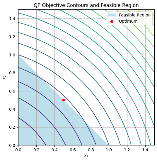
Output: Optimal value ≈ 0.75 at x ≈ [0.5, 0.5] (interior due to linear term). Visualization Plot the objective contours and feasible region:

import numpy as np
import matplotlib.pyplot as plt

x1 = np.linspace(0, 1.5, 100)
x2 = np.linspace(0, 1.5, 100)
X1, X2 = np.meshgrid(x1, x2)
Z = X1**2 + X2**2 + X1 + X2

plt.figure(figsize=(6, 6))
plt.contour(X1, X2, Z, levels=20, cmap='viridis')
plt.fill([0, 1, 0], [0, 0, 1], 'lightblue', alpha=0.8, label='Feasible Region')  # Simplified triangle
plt.scatter(0.5, 0.5, color='red', label='Optimum')
plt.xlabel('$x_1$')
plt.ylabel('$x_2$')
plt.title('QP Objective Contours and Feasible Region')
plt.legend()
plt.grid(True)
plt.show()

../_images/c79403ed7f6a878023704e7455a5f0e7dc36fd40a79318fe5c3ce13846025e92.png

For more complex QPs in engineering, use libraries like CVXPY (not in env, but extendable).

7.6 Linear least-squares#

Linear least-squares problems connect overdetermined algebraic systems (more equations than unknowns, from Chapter 4) to optimization by minimizing the residual norm, turning inconsistency into an underdetermined optimization over the solution space. This is key in data fitting, signal processing, and parameter estimation in space engineering (e.g., orbit determination from noisy measurements).

Connecting Overdetermined Systems to Underdetermined Optimization#

An overdetermined system $\mathbf{A} \mathbf{x} = \mathbf{b}$ (with $\mathbf{A} \in \mathbb{R}^{m \times n}$, $m > n$) often has no exact solution. Instead, solve the optimization problem:

\[\min_{\mathbf{x}} \| \mathbf{A} \mathbf{x} - \mathbf{b} \|_2^2,\]

which is underdetermined in the sense that we optimize over $\mathbf{x} \in \mathbb{R}^n$ without equality constraints, but the quadratic objective (with $\mathbf{Q} = 2\mathbf{A}^\top \mathbf{A}$) makes it a QP. The normal equations $\mathbf{A}^\top \mathbf{A} \mathbf{x} = \mathbf{A}^\top \mathbf{b}$ give the solution, but numerically, use QR or SVD for stability.

This bridges Chapter 4’s exact solves to optimization: Overdetermined system to minimize mismatch.

Basic Technique and State of the Art#

Basic technique: For unconstrained linear least-squares, use the pseudoinverse or decomposition.

QR decomposition: Factor $\mathbf{A} = \mathbf{Q} \mathbf{R}$, solve $\mathbf{R} \mathbf{x} = \mathbf{Q}^\top \mathbf{b}$.
SVD: $\mathbf{A} = \mathbf{U} \mathbf{\Sigma} \mathbf{V}^\top$, $\mathbf{x} = \mathbf{V} \mathbf{\Sigma}^+ \mathbf{U}^\top \mathbf{b}$ (robust to rank-deficiency).

State of the art libraries like LAPACK (via NumPy/SciPy) use these; for large-scale, iterative methods like LSQR (conjugate gradients for least-squares) handle sparsity. In machine learning, generalizations include regularized variants (e.g., Ridge: add $\lambda \| \mathbf{x} \|_2^2$).

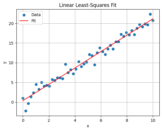
Python example: Fit line to noisy data (overdetermined).

import numpy as np
import matplotlib.pyplot as plt

# Overdetermined: m=50 points, n=2 params (slope, intercept)
x = np.linspace(0, 10, 50)
y = 2 * x + 1 + np.random.randn(50)  # Noisy data
A = np.vstack([x, np.ones_like(x)]).T  # Design matrix
b = y

# Solve least-squares
params, residuals, rank, s = np.linalg.lstsq(A, b, rcond=None)
print(f"Params: slope={params[0]:.2f}, intercept={params[1]:.2f}")

# Plot
plt.scatter(x, y, label='Data')
plt.plot(x, params[0]*x + params[1], 'r-', label='Fit')
plt.xlabel('x')
plt.ylabel('y')
plt.title('Linear Least-Squares Fit')
plt.legend()
plt.grid(True)
plt.show()

Params: slope=2.08, intercept=0.36

../_images/72692d5588d76ea6242cae4bbc4de7d548068560641bb5a6b1f7422544f7ff2a.png

7.7 Gradient-descent methods#

Gradient-descent (GD) methods solve unconstrained optimization problems by iteratively following the negative gradient, ideal for smooth, differentiable objectives. They set the stage for nonlinear optimization in Chapter 8 and ML applications like neural network training.

Formal Definition of Unconstrained Optimization Problems#

Definition: An unconstrained optimization problem is:

\[\min_{\mathbf{x} \in \mathbb{R}^n} f(\mathbf{x}),\]

where $f: \mathbb{R}^n \to \mathbb{R}$ is differentiable (often twice for convergence analysis). GD iterates:

\[\mathbf{x}_{k+1} = \mathbf{x}_k - \alpha_k \nabla f(\mathbf{x}_k),\]

with step size $\alpha_k > 0$ (fixed or line-searched).

Convergence requires Lipschitz continuity of $\nabla f$; for convex $f$, it reaches global minimum.

Variants: Momentum adds inertia, Nesterov accelerates; in Chapter 8, SGD handles noise.

Example: Basic Python Demonstration for Gradient Descent

Minimize $f(x) = x^2 + \sin(2\pi x)$ (from 7.1) using vanilla GD. Play with the step size $\alpha$ and starting point $x_0$ to see convergence behavior and gain a deep understanding of GD behavior on a nonconvex function with multiple local minima. The key concepts to understand are how the step size affects convergence speed and stability, and how the starting point can lead to different local minima without a basin of attraction (but also can escape shallow minima with a larger step size).

from ipywidgets import interact, FloatSlider

def f(x):
    return x**2 + np.sin(2 * np.pi * x)

def grad_f(x):
    return 2*x + 2*np.pi*np.cos(2*np.pi*x)


def gd_demo(alpha=0.01, x_start=1.5):
    x = x_start
    history = [x]
    for _ in range(100):
        x -= alpha * grad_f(x)
        history.append(x)

    t = np.linspace(-2, 2, 1000)
    plt.plot(t, f(t), label='$f(x)$')
    plt.plot(history, f(np.array(history)), 'ro-', label='GD Path')
    plt.xlabel('x')
    plt.ylabel('f(x)')
    plt.title(f'GD with α={alpha}, start={x_start}')
    plt.legend()
    plt.grid(True)
    plt.show()

interact(gd_demo, alpha=FloatSlider(min=0.001, max=0.1, step=0.001, value=0.01),
         x_start=FloatSlider(min=-2, max=2, step=0.1, value=1.5));

Lipschitz Continuity, Local and Global Minima#

While gradient-descent methods are powerful for unconstrained optimization, their behavior depends on properties of the objective function $f(\mathbf{x})$. Here, we formally define key concepts that influence convergence and solution quality.

Defintion: Lipschitz Continuity: A function $f: \mathbb{R}^n \to \mathbb{R}$ (or its gradient $\nabla f$) is Lipschitz continuous with constant $L > 0$ if, for all $\mathbf{x}, \mathbf{y}$ in the domain,$$\| f(\mathbf{x}) - f(\mathbf{y}) \| \leq L \| \mathbf{x} - \mathbf{y} \|.$$For gradients, this applies to $| \nabla f(\mathbf{x}) - \nabla f(\mathbf{y}) | \leq L | \mathbf{x} - \mathbf{y} |$ (Lipschitz gradient). This bounds how fast the function changes, ensuring step sizes like $\alpha < 1/L$ lead to convergence in GD.

Gradient descent converges to stationary points where $\nabla f(\mathbf{x}^*) = 0$. However, these points can be local minima, maxima, or saddle points, especially in nonconvex functions. Typically, we seek local minima, but global minima are ideal, gradient descent may get stuck in local minima:

Definition: Local Minimum: A point $\mathbf{x}^*$ is a local minimum if there exists a neighborhood $\mathcal{N}$ around $\mathbf{x}^*$ such that $f(\mathbf{x}^*) \leq f(\mathbf{x})$ for all $\mathbf{x} \in \mathcal{N}$. At a local minimum, $\nabla f(\mathbf{x}^*) = \mathbf{0}$ (first-order necessary condition), and the Hessian $\nabla^2 f(\mathbf{x}^*)$ is positive semi-definite.

A local minimum may or not be a global minimum, depending on the function’s landscape:

Definition: Global Minimum: A point $\mathbf{x}^*$ is a global minimum if $f(\mathbf{x}^*) \leq f(\mathbf{x})$ for all $\mathbf{x}$ in the domain. Convex functions guarantee any local minimum is global, but nonconvex functions may have multiple local minima.

Informally, recall the gradient descent example above on $f(x) = x^2 + \sin(2\pi x)$: Starting from different initial points (e.g., $x=1.5$ vs. $x=-1.5$) can lead to different paths and potentially converge to different local minima due to the function’s oscillations. This highlights how initial conditions affect outcomes in nonconvex landscapes.

We will explore these concepts in more depth in later chapters, particularly in the context of nonlinear optimization (Chapter 8) and global methods (Chapter 9), including convergence rates and strategies for escaping local minima.

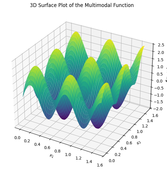
Example: Interactive Multimodal 2D Example

To experiment with gradient descent on a multimodal function (one with multiple local minima), consider $f(x_1, x_2) = \sin(3\pi x_1) + \sin(3\pi x_2) + 0.1(x_1^2 + x_2^2)$. This has several basins of attraction. Use the widget below to select a starting point $(x_1, x_2)$, adjust the step size $\alpha$, and observe the GD path on the contour plot. The red line shows the trajectory, illustrating how different starts lead to different minima.

import numpy as np
import matplotlib.pyplot as plt
from ipywidgets import interact, FloatSlider

min_x = 0
min_y = 0

# Define the multimodal function and gradient
def f(x1, x2):
    return np.sin(3 * np.pi * x1) + np.sin(3 * np.pi * x2) + 0.1 * (x1**2 + x2**2)

def grad_f(x1, x2):
    df_dx1 = 3 * np.pi * np.cos(3 * np.pi * x1) + 0.2 * x1
    df_dx2 = 3 * np.pi * np.cos(3 * np.pi * x2) + 0.2 * x2
    return np.array([df_dx1, df_dx2])

# GD function
def run_gd(start_x1, start_x2, alpha, max_iters=100):
    x = np.array([start_x1, start_x2])
    path = [x.copy()]
    for _ in range(max_iters):
        grad = grad_f(*x)
        x -= alpha * grad
        path.append(x.copy())
        if np.linalg.norm(grad) < 1e-4:
            break
    return np.array(path)

# Interactive plot
def plot_gd(start_x1=0.5, start_x2=0.5, alpha=0.01):
    path = run_gd(start_x1, start_x2, alpha)

    # Contour plot
    x1 = np.linspace(min_x, 1.5, 200)
    x2 = np.linspace(min_y, 1.5, 200)
    X1, X2 = np.meshgrid(x1, x2)
    Z = f(X1, X2)

    plt.figure(figsize=(8, 6))
    plt.contour(X1, X2, Z, levels=20, cmap='viridis', alpha=0.7)
    plt.colorbar(label='f(x1, x2)')
    plt.plot(path[:, 0], path[:, 1], 'r-', marker='o', markersize=3, label='GD Path')
    plt.scatter(path[0, 0], path[0, 1], color='green', s=100, label='Start')
    plt.scatter(path[-1, 0], path[-1, 1], color='black', s=100, label='End')
    plt.xlabel('$x_1$')
    plt.ylabel('$x_2$')
    plt.title('Gradient Descent on Multimodal Function')
    plt.legend()
    plt.grid(True)
    plt.show()

interact(plot_gd,
         start_x1=FloatSlider(min=min_x, max=1.5, step=0.05, value=0.7, description='Start x1:'),
         start_x2=FloatSlider(min=min_y, max=1.5, step=0.05, value=0.6, description='Start x2:'),
         alpha=FloatSlider(min=0.001, max=0.05, step=0.001, value=0.01, description='Alpha:'));

The plot below just shows the 3D surface of the multimodal function to visualize its landscape:

import numpy as np
import matplotlib.pyplot as plt
from mpl_toolkits.mplot3d import Axes3D

# Define the function
def f(x1, x2):
    return np.sin(3 * np.pi * x1) + np.sin(3 * np.pi * x2) + 0.1 * (x1**2 + x2**2)

# Generate grid
x1 = np.linspace(min_x, 1.5, 100)
x2 = np.linspace(min_y, 1.5, 100)
X1, X2 = np.meshgrid(x1, x2)
Z = f(X1, X2)

# Plot
fig = plt.figure(figsize=(10, 7))
ax = fig.add_subplot(111, projection='3d')
ax.plot_surface(X1, X2, Z, cmap='viridis', edgecolor='none')
ax.set_xlabel('$x_1$')
ax.set_ylabel('$x_2$')
ax.set_zlabel('$f(x_1, x_2)$')
ax.set_title('3D Surface Plot of the Multimodal Function')
plt.show()

../_images/cc60207762bc63d9fa214b6e1728d752176a4ab2a1e43b1b2b6da717895c3a4c.png

Basis	\(x_1\)	\(x_2\)	\(s_1\)	\(s_2\)	\(s_3\)	RHS
\(s_1\)	1	1	1	0	0	2
\(s_2\)	1	0	0	1	0	1.5
\(s_3\)	0	1	0	0	1	1
\(z\)	-1	-1	0	0	0	0

Basis	\(x_1\)	\(x_2\)	\(s_1\)	\(s_2\)	\(s_3\)	RHS
\(s_1\)	0	1	1	-1	0	0.5
\(x_1\)	1	0	0	1	0	1.5
\(s_3\)	0	1	0	0	1	1
\(z\)	0	-1	0	1	0	1.5

Basis	\(x_1\)	\(x_2\)	\(s_1\)	\(s_2\)	\(s_3\)	RHS
\(x_2\)	0	1	1	-1	0	0.5
\(x_1\)	1	0	-1	2	0	1
\(s_3\)	0	0	-1	1	1	0.5
\(z\)	0	0	1	0	0	2

Chapter 7: Convex and Linear Optimization

Contents

Chapter 7: Convex and Linear Optimization#

7.1 Optimization in general#

7.1.1 Formal Statement of the General Optimization Problem#

7.1.2 Brute Force Search: A Simple Visual Demonstration in Python#

Example: Brute force search

Example: Brute Force on a 2D Quadratic Function

7.2 Classification of common optimization problems#

7.3 Convexity#

Example: Python Demonstration of Convexity

7.4 Linear programming (LP)#

7.4.1 Simplex method#

Revised simplex method#

7.4.2 Interior point method#

Example: IPM steps

7.4.3 Dual Problem#

Geometric Interpretation#

7.4.4 Hybrid methods#

Basic Overview of HiGHS:#

7.5 Quadratic programming#

Example: Simple 2D Example

7.6 Linear least-squares#

Connecting Overdetermined Systems to Underdetermined Optimization#

Basic Technique and State of the Art#

7.7 Gradient-descent methods#

Formal Definition of Unconstrained Optimization Problems#

Example: Basic Python Demonstration for Gradient Descent

Lipschitz Continuity, Local and Global Minima#

Example: Interactive Multimodal 2D Example

Further reading#

Linear Programming#

Simplex and revised simplex method:#

HiGHS solver:#

Convex Optimization#

Gradient Descent Methods#