Tutorial: Simulation#
Part 1: Algebraic Solvers#
Non-linear solver exercises#
These exercises are designed to reinforce the concepts covered in Chapter 4, including linear and nonlinear solvers, conditioning, scaling, Jacobians, Hessians, and Newton methods.
Exercise 1: Computing Jacobians and Hessians Analytically and Numerically#
Objective: Practice deriving and approximating Jacobians and Hessians for nonlinear functions.
Start with the scalar function:
Use SymPy to compute the analytical Jacobian (gradient) and Hessian at \((x_1, x_2) = (1, \pi/2)\).
Approximate the Jacobian and Hessian numerically using finite differences (e.g., with scipy.optimize.approx_fprime for gradient, and a similar approach for Hessian).
Compare the results and discuss truncation vs. round-off errors in finite differences.
Hints: For numerical Hessian, finite-difference the gradient. Vary the step size \(\epsilon\) (e.g., 1e-6 to 1e-8) to observe error trade-offs.
The code below is a starting point with the symbolic and numerical coded in.
import sympy as sp
from scipy.optimize import approx_fprime
import numpy as np

# Analytical with SymPy
x1, x2 = sp.symbols('x1 x2')
f_analytical = x1**2 * sp.sin(x2) + sp.exp(x1 * x2)

# Numerical function
def f_num(x):
    return x[0]**2 * np.sin(x[1]) + np.exp(x[0] * x[1])

#
print(f"Expected result = [9.5562802  4.81047738]")
Expected result = [9.5562802 4.81047738]
Excercise 2: Vector-valued functions#
Next, repeat the exercise for the vector function:
# Analytical with SymPy
x1, x2 = sp.symbols('x1 x2')
f_analytical = [x1**2 * sp.sin(x2) + sp.exp(x1 * x2),
                x2**2 * sp.sin(x1) + sp.exp(x1 * x2)]

# Numerical function
def f_num(x):
    return [x[0]**2 * np.sin(x[1]) + np.exp(x[0] * x[1]),
            x[1]**2 * np.sin(x[0]) + np.exp(x[0] * x[1])]
Exercise 3: Implementing a Single Gauss-Newton Iteration#
3.1) Gradient descent step#
The purpose of this exercise is to gain intuition for the Gauss-Newton method through manual implementation and visualization.
For the nonlinear system \(\mathbf{F}(\mathbf{x}) = \begin{pmatrix} x_1 + x_2 - 3 \\ x_1^2 + x_2^2 - 5 \end{pmatrix} = \mathbf{0}\):
Start from \(\mathbf{x}_0 = (1, 1.5)\).
Compute the Jacobian \(\mathbf{J}(\mathbf{x}_0)\) analytically or numerically.
Solve for the search direction \(\mathbf{p}\) using the Gauss-Newton normal equations.
Update \(\mathbf{x}_1 = \mathbf{x}_0 + \mathbf{p}\) and evaluate \(\|\mathbf{F}(\mathbf{x}_1)\|\).
Visualize the contours of \(S(\mathbf{x}) = \frac{1}{2} \|\mathbf{F}(\mathbf{x})\|^2\) and plot the step.
Hints: Use Matplotlib for contour plots. Compare with scipy.optimize.least_squares.
# Definition of F(x) = 0:
def F(x):
    return np.array([x[0] + x[1] - 3,
                     x[0]**2 + x[1]**2 - 5])
3.2) Improving Gauss-Newton step with line search#
The above equation assumed that \(\alpha_k = 1\) in the line search:
When we have knowledge of the Hessian \(f''(x) = \nabla^2 f(x) = H_f(x)\in \mathbb{R}^{d\times d}\), we can obtain the classical Newton step (\(iff\) the Hessian is invertible)):
An operator that is closely related to the Hessian is the Laplacian operator, defined as the divergence of the gradient of a function. In multiple dimensions, the Laplacian is given by:
Because the Laplacian doesn’t need to be inverted, it can be used to approximate the Newton step and is more suitable to higher dimensional problems with a large number of entries in the Hessian matrix. Implement the following two steps to improve the Gauss-Newton method:
3.2.1) Pseudo-Newton step#
Use the Laplacian operator to approximate value of \(\alpha_k\).
3.2.2) Full Newton step#
Implement the full matrix multiplication to \(H^-1 \nabla f\) to compute the Newton step.
3.2.3) Compare the two methods#
Compare the performance of 3.2.1 and 3.2.2 on a contour plot, a good metric for this performance is to measure the reduction in the residual \(\|\mathbf{F}(\mathbf{x})\|\) after one iteration.
3.3) A full solver#
You now have the building blocks to implement a full Gauss-Newton solver. Implement the iterative procedure:
Initialize \(\mathbf{x}_0\).
While not converged:
Compute \(\mathbf{F}(\mathbf{x}_k)\) and \(\mathbf{J}(\mathbf{x}_k)\).
Solve for \(\mathbf{p}_k\).
Perform line search to find \(\alpha_k\).
Update \(\mathbf{x}_{k+1} = \mathbf{x}_k + \alpha_k \mathbf{p}_k\).
Choose any of the methods you developed in 3.2 and compare the convergence behavior (number of iterations, final residual) with scipy.optimize.fsolve using the same initial guess.
Below is a skeleton to get you started, but feel free to modify as needed.
def solve_gauss_newton(F, x0, tol=1e-6, max_iter=100):
    xk = x0
    for k in range(max_iter):
        # Compute F and J
        # Solve for pk
        #
        # Update x_k+1
        xk = xk + alpha_k * pk
        if np.linalg.norm(Fk) < tol:
            break
    return xk
Linear Solver Exercises#
Exercise 4: Analyzing Matrix Conditioning and Scaling#
The purpose of this exercise is to understand the impact of matrix conditioning on solution stability and explore scaling techniques to improve numerical accuracy.
Problem: Consider the linear system \(\mathbf{Ax} = \mathbf{b}\) where: $\(\mathbf{A} = \begin{pmatrix} 1 & 1 \\ 1 & 1.0001 \end{pmatrix}, \quad \mathbf{b} = \begin{pmatrix} 2 \\ 2.0001 \end{pmatrix}.\)$
Compute the condition number of \(\mathbf{A}\) using np.linalg.cond. Solve for \(\mathbf{x}\) and perturb \(\mathbf{b}\) by a small amount (e.g., add 0.001 to each element). Observe the change in \(\mathbf{x}\). Scale the rows of \(\mathbf{A}\) and \(\mathbf{b}\) to have unit norm (e.g., divide each row by its Euclidean norm) and repeat the process. Compare the condition numbers and solution sensitivities.
Hints: Use np.linalg.solve for solving. Discuss why scaling helps in ill-conditioned systems.
import numpy as np

# Define A and b
A = np.array([[1, 1], [1, 1.0001]])
b = np.array([2, 2.0001])

# Compute condition number
cond = np.linalg.cond(A)
print(f"Condition number: {cond}")

# Solve original system
x = np.linalg.solve(A, b)

# Perturb b and solve again
b_perturbed = b + 0.001
x_perturbed = np.linalg.solve(A, b_perturbed)
print(f"Relative change in x: {np.linalg.norm(x - x_perturbed) / np.linalg.norm(x)}")

# Scaling: Normalize rows
row_norms = np.linalg.norm(A, axis=1)
A_scaled = A / row_norms[:, np.newaxis]
b_scaled = b / row_norms

# Repeat condition and solves...
Condition number: 40002.00007491187
Relative change in x: 0.0007071067811864696
Excercise 6: Implementing and Comparing Gaussian Elimination vs. LU Decomposition#
In the excercise we want to demonstrate the relationship between Gaussian elimination (which you might remember from undergrad linear algebra classes) and LU decomposition, implement both from scratch, and compare their efficiency and stability for solving linear systems.
Consider the linear system \(\mathbf{Ax} = \mathbf{b}\) with:
1.Implement Gaussian elimination without pivoting to solve for \(\mathbf{x}\). Track the elimination steps and compute the effective upper triangular matrix. 2. Implement LU decomposition without pivoting (i.e., factor \(\mathbf{A} = \mathbf{LU}\), where \(\mathbf{L}\) has 1s on the diagonal). 3. Solve the system using the LU factors (forward substitution for \(\mathbf{Ly} = \mathbf{b}\), then back substitution for \(\mathbf{Ux} = \mathbf{y}\)). 4. Compare the results from both methods. Then, test with multiple \(\mathbf{b}\) vectors (e.g., add \(\mathbf{b}_2 = [1, 2, 3]^\top\)) and measure computation time using %timeit in Jupyter. 5. Introduce a small perturbation to \(\mathbf{A}\) (e.g., add 1e-10 to one element) and discuss stability differences. Optionally, add partial pivoting to both implementations and recompare.
Hints:
In Gaussian elimination, augment \(\mathbf{A}\) with \(\mathbf{b}\) and perform row operations.
For LU, store multipliers in \(\mathbf{L}\) below the diagonal during elimination.
Use NumPy for array operations but avoid built-in solvers like np.linalg.solve—implement the algorithms manually for learning.
Reference SciPy’s scipy.linalg.lu_factor for validation, but explain why it’s more robust.
Both methods should yield \(\mathbf{x} \approx [1, 2, 2]^\top\). LU is more efficient for multiple \(\mathbf{b}\) since factorization is done once. Without pivoting, both can fail on singular/ill-conditioned matrices—discuss how partial pivoting (e.g., swapping rows) improves stability, mirroring real-world implementations like scipy.linalg.lu.
The full algorithms are provided below to get you started:
Gaussian Elimination Algorithm#
Gaussian elimination transforms the augmented matrix \([\mathbf{A} | \mathbf{b}]\) into row echelon form (upper triangular) through row operations, then solves via back substitution. For a system \(\mathbf{Ax} = \mathbf{b}\) where \(\mathbf{A} \in \mathbb{R}^{n \times n}\), the algorithm proceeds as follows (without pivoting for simplicity):
Forward Elimination Phase: 1.1 For each pivot row \(k = 1\) to \(n-1\): For each row \(i = k+1\) to \(n\): Compute the multiplier: \(m_{ik} = \frac{a_{ik}}{a_{kk}}\) Update row \(i\): \(a_{ij} \leftarrow a_{ij} - m_{ik} a_{kj}\) for \(j = k\) to \(n\) Update right-hand side: \(b_i \leftarrow b_i - m_{ik} b_k\)
This results in an upper triangular matrix \(\mathbf{U}\) and updated \(\mathbf{b}'\).Symbolically, the elimination step for element \(a_{ij}\) (with \(i > k, j \geq k\)) is:$\(a_{ij}^{(k)} = a_{ij}^{(k-1)} - \frac{a_{ik}^{(k-1)}}{a_{kk}^{(k-1)}} a_{kj}^{(k-1)}\)\(where superscript \)(k)\( denotes after the \)k\(-th elimination step. 1.2 Back Substitution Phase: Starting from the last equation:\)\(x_n = \frac{b_n'}{u_{nn}}\)\(Then for \)i = n-1\( down to \)1\(:\)\(x_i = \frac{b_i' - \sum_{j=i+1}^n u_{ij} x_j}{u_{ii}}\)$
This method has a time complexity of \(O(n^3)\) due to the nested loops in elimination.
LU Decomposition Algorithm LU decomposition factors \(\mathbf{A}\) into a lower triangular matrix \(\mathbf{L}\) (with 1s on the diagonal) and an upper triangular matrix \(\mathbf{U}\), such that \(\mathbf{A} = \mathbf{LU}\). This is equivalent to Gaussian elimination but stores the multipliers in \(\mathbf{L}\). For solving \(\mathbf{Ax} = \mathbf{b}\), first solve \(\mathbf{Ly} = \mathbf{b}\) (forward substitution), then \(\mathbf{Ux} = \mathbf{y}\) (back substitution).
2.1 Factorization Phase (Doolittle’s Algorithm, without pivoting): Initialize \(\mathbf{L} = \mathbf{I}\) (identity) and \(\mathbf{U} = \mathbf{A}\).For each column \(k = 1\) to \(n\): For the upper part (\(j = k\) to \(n\)): \(u_{kj} = a_{kj}\) (already set) For the multipliers (\(i = k+1\) to \(n\)): $\(l_{ik} = \frac{u_{ik}}{u_{kk}}, \quad u_{ij} \leftarrow u_{ij} - l_{ik} u_{kj} \quad \forall j \geq k\)\( More formally, for \)k = 1\( to \)n\(:\)\(u_{kk} = a_{kk} - \sum_{m=1}^{k-1} l_{km} u_{mk}\)\(For \)j = k+1\( to \)n\(:\)\(u_{kj} = a_{kj} - \sum_{m=1}^{k-1} l_{km} u_{mj}\)\(For \)i = k+1\( to \)n\(:\)\(l_{ik} = \frac{1}{u_{kk}} \left( a_{ik} - \sum_{m=1}^{k-1} l_{im} u_{mk} \right)\)\( 2.2 Forward Substitution (\)\mathbf{Ly} = \mathbf{b}\():\)\(y_1 = \frac{b_1}{l_{11}} = b_1 \quad (\text{since } l_{11} = 1)\)\(For \)i = 2\( to \)n\(:\)\(y_i = b_i - \sum_{j=1}^{i-1} l_{ij} y_j\)\( 2.3 Back Substitution (\)\mathbf{Ux} = \mathbf{y}$): Identical to Gaussian elimination’s back substitution phase.
LU decomposition also has \(O(n^3)\) complexity for factorization but allows efficient reuse for multiple \(\mathbf{b}\) vectors (each solve is \(O(n^2)\)). Note on Pivoting: In practice, partial pivoting is added to both methods for numerical stability, swapping rows to select the largest pivot and avoid division by small numbers. This modifies the algorithms to produce \(\mathbf{PA} = \mathbf{LU}\) where \(\mathbf{P}\) is a permutation matrix.
Exercise 7: Comparing Direct Linear Solvers (LU vs. SVD)#
In this exertcise we evaluate stability and performance of direct solvers for ill-conditioned systems. Problem: Generate a Hilbert matrix \(\mathbf{H}_n\) (ill-conditioned) of size \(n=10\): $\(H_{ij} = \frac{1}{i + j - 1}\)$
Solve \(\mathbf{Hx} = \mathbf{b}\) (let \(\mathbf{b} = \mathbf{H} \cdot \mathbf{1}\), true \(\mathbf{x} = \mathbf{1}\)) using LU decomposition (scipy.linalg.lu_solve) and SVD (np.linalg.pinv). Perturb \(\mathbf{b}\) slightly and compare recovered \(\mathbf{x}\) errors. Measure computation time for increasing \(n\).
Hints: Use scipy.linalg.lu_factor for LU. SVD is more robust for rank-deficient cases.
Exercise 8: Implementing and Testing Gauss-Seidel Iteration#
Objective: Implement an iterative solver and analyze convergence conditions. Problem: Solve the system from the chapter example: $\(\mathbf{A} = \begin{pmatrix} 4 & -1 & 0 \\ -1 & 4 & -1 \\ 0 & -1 & 4 \end{pmatrix}, \quad \mathbf{b} = \begin{pmatrix} 2 \\ 3 \\ 2 \end{pmatrix}.\)$
Implement Gauss-Seidel with a tolerance of 1e-6 and max 100 iterations. Test on a non-diagonally dominant matrix (e.g., swap rows) and observe divergence. Add SOR with \(\omega = 1.2\) and compare iteration counts.
Hints: Check diagonal dominance: \(|a_{ii}| \geq \sum_{j \neq i} |a_{ij}|\).
Part 2: ODE/DAE integrators#
Exercise 1: Forward Euler for a Simple Orbital Decay Model (Basic ODE)#
1.1 Forward Euler simulation#
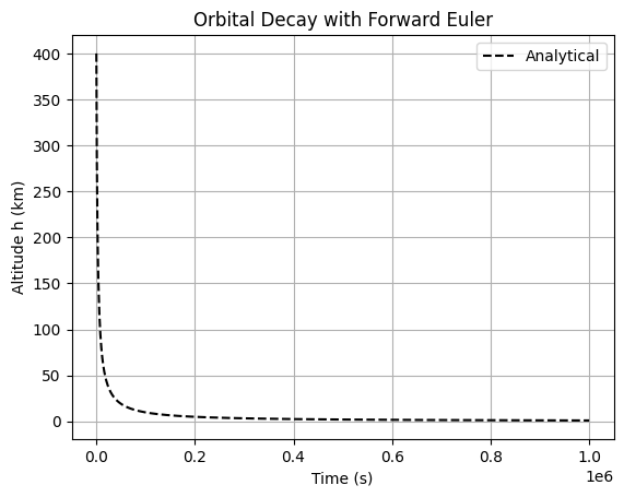
Simulate the altitude decay of a low-Earth orbit satellite due to atmospheric drag using the scalar ODE \(\frac{dh}{dt} = -k h^2\) (simplified drag model), where \(h(t)\) is altitude, \(k = 10^{-6}\) km⁻¹ s⁻¹ is a drag coefficient. Initial condition: \(h(0) = 400\) km. Integrate over \(t \in [0, 10^6]\) s. Implement forward Euler; explore step size effects on accuracy/stability. Compare to analytical solution \(h(t) = \frac{h_0}{1 + k h_0 t}\).
1.2 Error analysis and stability#
Implement an error function (\(e.g. ||h_numerical - h_analytical||\)) Try much larger dt values and comment on stability.
import numpy as np
import matplotlib.pyplot as plt

# Parameters
h0 = 400.0  # km
k = 1e-6    # km^-1 s^-1
t_f = 1e6   # s
dt = 1e1  # Note: higher values can result in overflow errors

#TODO: Implement:
# The ODE function dh/dt
def dhdt(t, h, k):
    pass
# Data containers to save numerical solution e.g. t_num = [], h_num = []:

# A forward Euler integration loop (while or for loop)


# Analytical solution for comparison
t_anal = np.linspace(0, t_f, 1000)
h_anal = h0 / (1 + k * h0 * t_anal)

# Plot
#plt.plot(t_num, h_num, label='Forward Euler')
plt.plot(t_anal, h_anal, 'k--', label='Analytical')
plt.xlabel('Time (s)')
plt.ylabel('Altitude h (km)')
plt.title('Orbital Decay with Forward Euler')
plt.legend()
plt.grid()
plt.show()

# TODO: Compute max error; test dt = 1e3, 1e5; discuss stability.
Exercise 2: Implicit Euler for a Stiff Reaction Control System (Stiffness)#
2.1 Implicit Euler simulation#
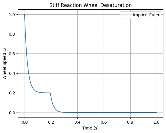
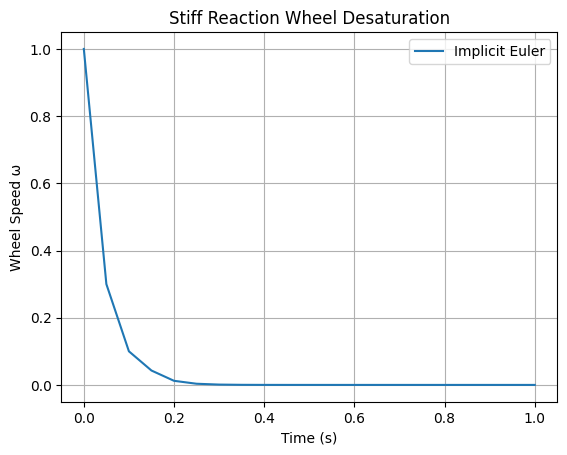
Model a spacecraft’s reaction wheel desaturation using thrusters: \(\frac{d\omega}{dt} = -50 \omega + u(t)\), where \(\omega\) is wheel speed (stiff due to fast torque response), \(u(t)\) is control input (e.g., step function). Initial \(\omega(0) = 10\). Integrate over \(t \in [0, 1]\) with \(u(t) = 1\) for \(t < 0.2\), else 0. Implement implicit Euler with fsolve; demonstrate stability for large dt where forward Euler fails.
2.2 Stability analysis#
Analyze eigenvalues for stiffness.
from scipy.optimize import fsolve

# ODE: dω/dt = -50 ω + u(t)
def u(t):
    return 10 if t < 0.2 else 0

def dωdt(t, ω):
    return -50 * ω + u(t)

# Implicit Euler loop (dt=0.05, unstable for forward)
ω = 1.0
t = 0.0
t_f = 1.0
dt = 0.005  # Play with lower values
t_values = [t]
ω_values = [ω]
while t < t_f:
    pass
    t += dt
    # Implement implicit Euler step using fsolve

# Plot (add forward Euler for comparison, expect oscillations)
plt.plot(t_values, ω_values, label='Implicit Euler')
plt.xlabel('Time (s)')
plt.ylabel('Wheel Speed ω')
plt.title('Stiff Reaction Wheel Desaturation')
plt.legend()
plt.grid()
plt.show()

# TODO: Compute Jacobian eigenvalue; test dt=0.1.
# Solution

from scipy.optimize import fsolve

# ODE: dω/dt = -50 ω + u(t)
def u(t):
    return 10 if t < 0.2 else 0

def dωdt(t, ω):
    return -50 * ω + u(t)

# Implicit Euler loop (dt=0.05, unstable for forward)
ω = 1.0
t = 0.0
t_f = 1.0
dt = 0.005  # Play with lower values
t_values = [t]
ω_values = [ω]
while t < t_f:
    t_next = t + dt
    def res(ω_next):
        return ω_next - ω - dt * dωdt(t_next, ω_next)
    ω = fsolve(res, ω)[0]
    t = t_next
    t_values.append(t)
    ω_values.append(ω)

# Plot (add forward Euler for comparison, expect oscillations)
plt.plot(t_values, ω_values, label='Implicit Euler')
plt.xlabel('Time (s)')
plt.ylabel('Wheel Speed ω')
plt.title('Stiff Reaction Wheel Desaturation')
plt.legend()
plt.grid()
plt.show()

# TODO: Compute Jacobian eigenvalue; test dt=0.1.
/tmp/ipykernel_2511/1940925007.py:23: RuntimeWarning: The iteration is not making good progress, as measured by the
 improvement from the last ten iterations.
  ω = fsolve(res, ω)[0]
# SOLUTION:
from scipy.optimize import fsolve

# ODE: dω/dt = -50 ω + u(t)
def u(t):
    return 1 if t < 0.2 else 0

def dωdt(t, ω):
    return -50 * ω + u(t)

# Implicit Euler loop (dt=0.05, unstable for forward)
ω = 1.0
t = 0.0
t_f = 1.0
dt = 0.05
t_values = [t]
ω_values = [ω]
while t < t_f:
    t_next = t + dt
    def res(ω_next):
        return ω_next - ω - dt * dωdt(t_next, ω_next)
    ω = fsolve(res, ω)[0]
    t = t_next
    t_values.append(t)
    ω_values.append(ω)

# Plot (add forward Euler for comparison, expect oscillations)
plt.plot(t_values, ω_values, label='Implicit Euler')
plt.xlabel('Time (s)')
plt.ylabel('Wheel Speed ω')
plt.title('Stiff Reaction Wheel Desaturation')
plt.legend()
plt.grid()
plt.show()

# Tasks: Add forward Euler; compute Jacobian eigenvalue; test dt=0.1.
/tmp/ipykernel_2511/860934069.py:22: RuntimeWarning: The iteration is not making good progress, as measured by the
 improvement from the last ten iterations.
  ω = fsolve(res, ω)[0]
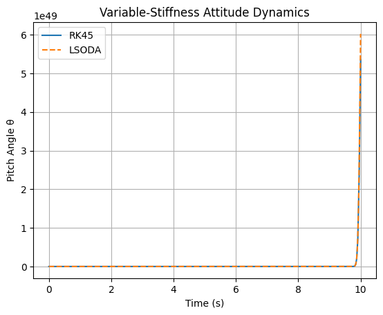
Problem 3: Runge-Kutta vs. LSODA for Variable-Stiffness Attitude Dynamics (Advanced Solvers)#
Simulate a spacecraft’s pitch angle \(\theta\) with variable damping: $\(\frac{d^2\theta}{dt^2} + b(t)\)$
recast as first-order system. \(b(t) = 1 + 50 \sin(2\pi t)\) (time-varying stiffness).
Initial conditions: \(\theta(0)=1\), \(\dot{\theta}(0)=0\).
Integrate over \(t \in [0, 10]\) using both RK45 and LSODA from scipy.integrate.solve_ivp, then compare the number of steps taken by each solver (e.g. print len(sol_rk.t) vs len(sol_lsoda.t); discuss switching.
from scipy.integrate import solve_ivp

t_range = [0, 10]
y0 = [1.0, 0.0]

def b(t):
    return 1 + 50 * np.sin(2 * np.pi * t)

def dydt(t, y):
    #TODO:
    return


# Solve with using solve_ivp with `method=RK45` and `method=LSODA` e.g. sol_rk = solve_ivp(ode, t_range, y0, method='RK45')
sol_rk = None
sol_lsoda = None

# Plot θ
#plt.plot(sol_rk.t, sol_rk.y[0], label='RK45')
#plt.plot(sol_lsoda.t, sol_lsoda.y[0], '--', label='LSODA')
plt.xlabel('Time (s)')
plt.ylabel('Pitch Angle θ')
plt.title('Variable-Stiffness Attitude Dynamics')
plt.legend()
plt.grid()
plt.show()

# Tasks: Print len(sol_rk.t) vs len(sol_lsoda.t); discuss switching.
/tmp/ipykernel_2511/9301123.py:25: UserWarning: No artists with labels found to put in legend.  Note that artists whose label start with an underscore are ignored when legend() is called with no argument.
  plt.legend()
# SOLUTION part 1:
from scipy.integrate import solve_ivp

def ode(t, y):
    θ, dθ = y
    b = 1 + 50 * np.sin(2 * np.pi * t)
    k = 1.0
    return [dθ, -b * dθ - k * θ]

y0 = [1.0, 0.0]
sol_rk = solve_ivp(ode, [0, 10], y0, method='RK45')
sol_lsoda = solve_ivp(ode, [0, 10], y0, method='LSODA')

# Plot θ
plt.plot(sol_rk.t, sol_rk.y[0], label='RK45')
plt.plot(sol_lsoda.t, sol_lsoda.y[0], '--', label='LSODA')
plt.xlabel('Time (s)')
plt.ylabel('Pitch Angle θ')
plt.title('Variable-Stiffness Attitude Dynamics')
plt.legend()
plt.grid()
plt.show()

# Tasks: Print len(sol_rk.t) vs len(sol_lsoda.t); discuss switching.
# Solution part 2:
len(sol_rk.t), len(sol_lsoda.t)
(271, 989)
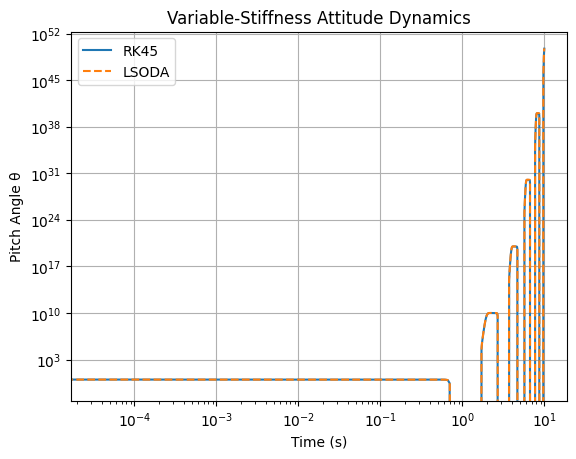
Note that sol_rk.t < sol_lsoda.t
plt.loglog(sol_rk.t, sol_rk.y[0], label='RK45')
plt.loglog(sol_lsoda.t, sol_lsoda.y[0], '--', label='LSODA')
plt.xlabel('Time (s)')
plt.ylabel('Pitch Angle θ')
plt.title('Variable-Stiffness Attitude Dynamics')
plt.legend()
plt.grid()
plt.show()
Problem 4: Index-1 DAE for Constrained Satellite Motion (DAEs)#
Model a tethered satellite system as index-1 DAE:
where \(L=100\) m, \(g=9.81\) m/s². Initial: \(y_1(0)=0\), \(y_2(0)=L\). Objectives: Implement using solve_ivp on reduced ODE (solve constraint for y); compare to full DAE solve with mass matrix.
# Reduced ODE after solving constraint for y = sqrt(L^2 - x^2)
import numpy as np

# Parameters
L = 100.0  # m
g = 9.81  # m/s^2

# Implement DAE system solving for dydt:


#sol = solve_ivp(dydt, [0, 10], [0, 1], method='LSODA')

# Plot y_1(t), y_1(t)
#plt.plot(sol.t, sol.y[0], label='y_1(t)')
#plt.plot(sol.t, np.sqrt(100**2 - sol.y[0]**2), label='y2(t)')
plt.xlabel('Time (s)')
plt.ylabel('Position (m)')
plt.title('Index-1 DAE: Tethered Satellite')
plt.legend()
plt.grid()
plt.show()

# Tasks: Implement full DAE with mass matrix in solve_ivp; check constraint violation.
/tmp/ipykernel_2511/2701594461.py:19: UserWarning: No artists with labels found to put in legend.  Note that artists whose label start with an underscore are ignored when legend() is called with no argument.
  plt.legend()
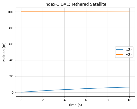
# SOLUTION:
# Reduced ODE after solving constraint for y = sqrt(L^2 - x^2)
def ode_reduced(t, z):  # z = [x, v]
    x, v = z
    L = 100.0
    g = 9.81
    y = np.sqrt(L**2 - x**2)
    dvdt = -g * y / L * (v / y)  # Simplified; derive properly
    return [v, dvdt]

sol = solve_ivp(ode_reduced, [0, 10], [0, 1], method='LSODA')

# Plot x(t), y(t)
plt.plot(sol.t, sol.y[0], label='x(t)')
plt.plot(sol.t, np.sqrt(100**2 - sol.y[0]**2), label='y(t)')
plt.xlabel('Time (s)')
plt.ylabel('Position (m)')
plt.title('Index-1 DAE: Tethered Satellite')
plt.legend()
plt.grid()
plt.show()

# Tasks: Implement full DAE with mass matrix in solve_ivp; check constraint violation.
(Optional) Problem 5: Symplectic Integrator for Long-Term Orbital Stability (Expanded)#
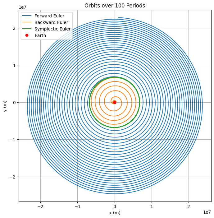
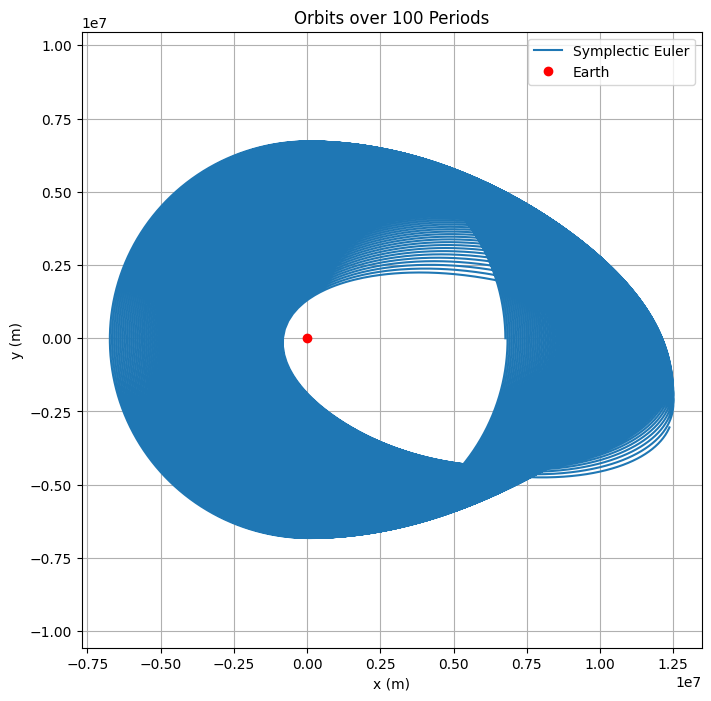
In this exercise we will use the Verlet (leapfrog) integrator to simulate an unperturbed two-body orbit (circular) over 100 orbital periods. For simplicity, use the 2D restricted two-body problem for a satellite around Earth: position \(\mathbf{q} = (x, y)\), momentum \(\mathbf{p} = (v_x, v_y)\) (unit mass), with equations \(\dot{\mathbf{q}} = \mathbf{p}\), \(\dot{\mathbf{p}} = -\frac{\mu}{r^3} \mathbf{q}\), where \(r = \|\mathbf{q}\|\) and \(\mu = 3.986 \times 10^{14}\) m³/s² (Earth). Initial conditions for circular Low Earth Orbit (LEO) at radius \(r_0 = 6771\) km: \(x(0) = r_0\), \(y(0) = 0\), \(v_x(0) = 0\), \(v_y(0) = \sqrt{\mu / r_0}\). This is a Hamiltonian system, periodic with constant energy \(E = \frac{1}{2} \|\mathbf{p}\|^2 - \frac{\mu}{r}\). We expect no decay in the orbit radius or energy over time.
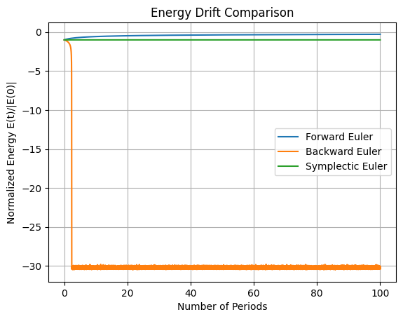
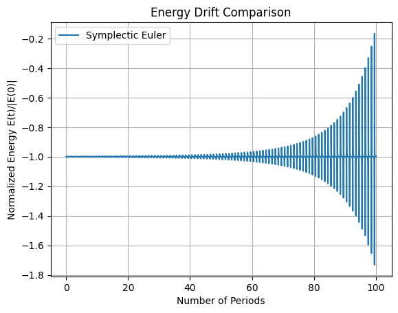
The simulation below shows the implementation of three integrators: Forward Euler, Backward Euler (implicit), and Verlet. We then compare their orbital paths and energy conservation over 100 orbital periods. In this exercise we want to gain insight into the difference between physical and numerical stability. In particular, we expect the symplectic Verlet integrator to conserve energy much better over long times compared to the non-symplectic Euler methods. We expect the Forward Euler to gain energy (orbit spirals out) and Backward Euler to lose energy (orbit spirals in). It’s important to think about why this is the case in terms of the numerical properties of the integrators.
import numpy as np
from scipy.optimize import fsolve
import matplotlib.pyplot as plt

# Parameters
mu = 3.986e14  # m^3/s^2
r0 = 6771000.0  # m (LEO)
v0 = np.sqrt(mu / r0)
T = 2 * np.pi * np.sqrt(r0**3 / mu)  # Orbital period ~5500 s
t_f = 100 * T  # 100 periods
dt = 10.0  # s

# Initial state y = [x, y, vx, vy]
y0 = np.array([r0, 0.0, 0.0, v0])

# ODE function f(y, mu) = dy/dt = [vx, vy, -mu x / r^3, -mu y / r^3]
def dydt(y, mu):
    x, y_pos, vx, vy = y
    r = np.sqrt(x**2 + y_pos**2)
    ax = -mu * x / r**3
    ay = -mu * y_pos / r**3
    return np.array([vx, vy, ax, ay])

# Data storage function
def simulate(integrator, label):
    t = 0.0
    y = y0.copy()
    t_values = [t]
    y_values = [y.copy()]
    E_values = [0.5 * (y[2]**2 + y[3]**2) - mu / np.linalg.norm(y[:2])]  # Initial E
    while t < t_f:
        y = integrator(y, dt, mu)
        t += dt
        y_values.append(y.copy())
        t_values.append(t)
        r = np.linalg.norm(y[:2])
        E = 0.5 * (y[2]**2 + y[3]**2) - mu / r
        E_values.append(E)
    return np.array(t_values), np.array(y_values), np.array(E_values)

# Forward Euler
def forward_euler(y, dt, mu):
    return y + dt * dydt(y, mu)

# Backward Euler (implicit)
def backward_euler(y, dt, mu):
    def res(y_next):
        return y_next - y - dt * dydt(y_next, mu)
    return fsolve(res, y)

# Symplectic Euler (momentum-first: update p using current q, then q using new p)
def symplectic_euler(y, dt, mu):
    accel = dydt(y, mu)[2:]  # Acceleration from current state (depends on q)
    p_new = y[2:] + dt * accel
    q_new = y[:2] + dt * p_new
    return np.concatenate([q_new, p_new])

# Simulate all
t_fwd, y_fwd, E_fwd = simulate(forward_euler, 'Forward Euler')
t_bwd, y_bwd, E_bwd = simulate(backward_euler, 'Backward Euler')
t_sym, y_sym, E_sym = simulate(symplectic_euler, 'Symplectic Euler')

# Plot orbits
plt.figure(figsize=(8, 8))
plt.plot(y_fwd[:, 0], y_fwd[:, 1], label='Forward Euler')
plt.plot(y_bwd[:, 0], y_bwd[:, 1], label='Backward Euler')
plt.plot(y_sym[:, 0], y_sym[:, 1], label='Symplectic Euler')
plt.plot(0, 0, 'ro', label='Earth')
plt.xlabel('x (m)')
plt.ylabel('y (m)')
plt.title('Orbits over 100 Periods')
plt.axis('equal')
plt.legend()
plt.grid()
plt.show()

# Plot energy
plt.figure()
plt.plot(t_fwd / T, E_fwd / abs(E_fwd[0]), label='Forward Euler')  # Normalized
plt.plot(t_bwd / T, E_bwd / abs(E_bwd[0]), label='Backward Euler')
plt.plot(t_sym / T, E_sym / abs(E_sym[0]), label='Symplectic Euler')
plt.xlabel('Number of Periods')
plt.ylabel('Normalized Energy E(t)/|E(0)|')
plt.title('Energy Drift Comparison')
plt.legend()
plt.grid()
plt.show()
/tmp/ipykernel_2511/3472954495.py:49: RuntimeWarning: The iteration is not making good progress, as measured by the
 improvement from the last ten iterations.
  return fsolve(res, y)
/tmp/ipykernel_2511/3472954495.py:49: RuntimeWarning: The iteration is not making good progress, as measured by the
 improvement from the last five Jacobian evaluations.
  return fsolve(res, y)
Tasks:
5.1 Analysis of Jacobian and Eigenvalues#
Compute the Jacobian matrix \(\mathbf{J} = \frac{\partial \mathbf{f}}{\partial \mathbf{y}}\) for the state vector \(\mathbf{y} = [x, y, v_x, v_y]^\top\), where \(\mathbf{f}(\mathbf{y}) = [v_x, v_y, -\mu x / r^3, -\mu y / r^3]^\top\). Evaluate it symbolically or numerically at a point on the circular orbit (e.g., initial condition). Compute eigenvalues to classify the fixed point (origin) or orbital stability: expect pure imaginary eigenvalues indicating a center (elliptic fixed point in linearized sense, leading to periodic motion without decay).
5.2 Implementing and Comparing Integrators#
In the above code we have implement forward Euler, backward (implicit) Euler, and Verlet integrators. Simulate over 100 orbital periods (\(T \approx 2\pi \sqrt{r_0^3 / \mu} \approx 5500\) s, so \(t_f = 100 T \approx 5.5 \times 10^5\) s). The first plot shows the position of the orbits over time, the second plot is the total energy \(E(t)\) for each method over time. Discuss why forward and backward Euler show artificial decay (numerical dissipation), while Verlet preserves energy with bounded oscillations (no long-term drift).
Additionally, experiment with different time step sizes (e.g., dt = 1 s, 10 s, 100 s) and observe how the energy conservation and orbit stability change for each integrator. Discuss the trade-offs between accuracy, stability, and computational cost for each method in the context of long-term orbital simulations.
5.3 Non-conservative systems#
What would happen if you added a small perturbation to the force function to simulate a non-conservative effect (e.g., atmospheric drag)? Modify the force function to include a small constant term (e.g., add a small - 1e-2 friction to the force function in the x or y directions) and rerun the simulation. Discuss how each integrator behaves in this non-conservative scenario, particularly focusing on energy dissipation and orbit decay. Compare only the symplectic integrator for clarity.
# Solution 5.1: Jacobian and Eigenvalues
def jacobian(y, mu):
    x, y_pos, vx, vy = y
    r = np.sqrt(x**2 + y_pos**2)
    r3 = r**3
    r5 = r**5
    J = np.zeros((4, 4))
    J[0, 2] = 1
    J[1, 3] = 1
    J[2, 0] = -mu / r3 + 3 * mu * x**2 / r5
    J[2, 1] = 3 * mu * x * y_pos / r5
    J[3, 0] = J[2, 1]  # Symmetric
    J[3, 1] = -mu / r3 + 3 * mu * y_pos**2 / r5
    return J

J = jacobian(y0, mu)
eigvals = np.linalg.eigvals(J)
print("Eigenvalues:", eigvals)  # Expect complex with zero real part for center
Eigenvalues: [ 0.00160252+0.j         -0.00160252+0.j          0.        +0.00113316j
  0.        -0.00113316j]
# Solution 5.2 is already included in the main simulation code above. Verlet integrators conserve the total energy and rotational momentum over time while the Euler methods do not.
# Solution 5.3

# ODE function f(y, mu) = dy/dt = [vx, vy, -mu x / r^3, -mu y / r^3]
def dydt(y, mu):
    x, y_pos, vx, vy = y
    r = np.sqrt(x**2 + y_pos**2)
    ax = -mu * x / r**3
    ay = -mu * y_pos / r**3 - 1e-2
    return np.array([vx, vy, ax, ay])

# Simulate all
t_fwd, y_fwd, E_fwd = simulate(forward_euler, 'Forward Euler')
##t_bwd, y_bwd, E_bwd = simulate(backward_euler, 'Backward Euler')
t_sym, y_sym, E_sym = simulate(symplectic_euler, 'Symplectic Euler')

# Plot orbits
plt.figure(figsize=(8, 8))
plt.plot(y_sym[:, 0], y_sym[:, 1], label='Symplectic Euler')
plt.plot(0, 0, 'ro', label='Earth')
plt.xlabel('x (m)')
plt.ylabel('y (m)')
plt.title('Orbits over 100 Periods')
plt.axis('equal')
plt.legend()
plt.grid()
plt.show()

# Plot energy
plt.figure()
plt.plot(t_sym / T, E_sym / abs(E_sym[0]), label='Symplectic Euler')
plt.xlabel('Number of Periods')
plt.ylabel('Normalized Energy E(t)/|E(0)|')
plt.title('Energy Drift Comparison')
plt.legend()
plt.grid()
plt.show()
#
Part 3: PDE solvers#
Exercise 1: Tubular reactors: extended heat equation for cylindrical coordinates#
1.1 Heat rod#
Change the initial conditions of Example 1 from the course notes to the following temperature profile \(u(x, 0) = 298 + 1000 x^2\). Comment on the effect of the initial gradient on the transient process. (5 min) \(~\\ ~\)
Increase the time discretization \(\Delta t\) in Example by a factor of 10.
Comment on the output of the simulation. (5 min)
Prove that the series is divergent. (10 min) \(~\\ ~\)
1.2 Symmetric coordinates in 2D reactors#
A plug flow reactor was operating a cold water run when the pumps broke down stopping all flows including the reactor water and steam duties in the heat jacket. The reactor has intial steady state temperature profile \( u(r, z, 0) = 298 + 200 \left( \frac{z}{L}\right)^{0.1} + 50 \sqrt{\frac{r}{R}}~\). It is known that axial symmetry may be assumed \(\left(\frac{\partial u}{\partial \Phi} = 0\right)\). The reactor has a length of 6 m and a radius of 0.3 m. On the boundaries heat (but no mass) is exchanged with the water left in the steam jacket as well as through the closed valves to the up and downstream stationary water in the reactor inlet and outlet. The heat jacket steam cools as heat is lost to the environment. The convection resistance between the heat jacket and the reactor is neglible and the boundary has the known space-time dependency \(u(R, z, t) = 298 + 250 \sqrt{\frac{z}{L}} e^{-5 \times 10^{-6} t}\). The upstream water is a constant temperature resevoir at 298 K while the downstream water ungergoes cooling of its own and has another space-time dependency \(u_{\infty, L}(r, t) = 298 + \left(200 + 50 \sqrt{\frac{r}{R}} \right) e^{-5 \times 10^{-6} t}\). The convection coefficient at the reactor inlets is approximately 300 \(~\textrm{W} \textrm{m}^{-2} \textrm{K}^{-1}\). Water has a thermal diffusivity of \(0.143 \times 10^{-6} \textrm{m}^2 \textrm{s}^{-1}\). As a first estimate the all physical parameters are considered constant.
Simulate for 60 hours of real time.
HINT: Use a heat transfer book reference for finding the cylindrical coordinate system before discretization.
1.3 Radiation (non-homogenous PDEs)#
The water used in the PFR in Example 2 is contaminated with radiation producing heat at a constant \(\dot{e}_{gen} = 1100000~\textrm{W}~\textrm{m}^{-3}\) (constant \(\rho c_p\)). Add the energy generation term \(\frac{\dot{e}_{gen}}{\kappa}\) with \(\kappa = 0.6~\textrm{W}~\textrm{m}^{-1}~\textrm{K}^{-1}\) to the PDE in the code (ignore energy generation on the boundaries) and simulate for 400 hours. (45 min)
HINT: Consider the total amount of energy generated in a discrete finite volume, in cylindrical cooridates this will vary with \(r\). Build a matrix with the volume of each discrete element \(i, j\) and use normal matrix algebra to add this term to the heat equation. \(~\\ ~\)
1.4 Real conductivity (non-linear PDEs)#
In example 2 we assumed a constant conductivity coefficient. Instead use a temperature dependent function. Note that you need to rederive the difference equation since the temperature at a discrete element varies in with the spatial coordinates). The following code snippet demonstrates how to construct a temperature dependent relation for conductivity: (60 min)
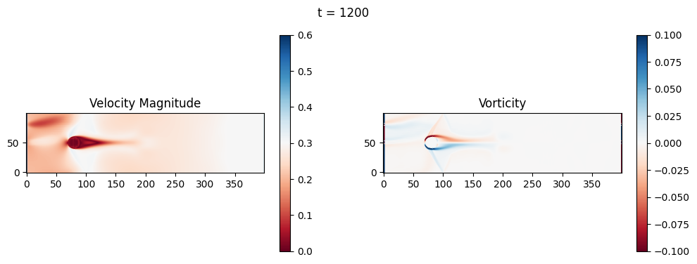
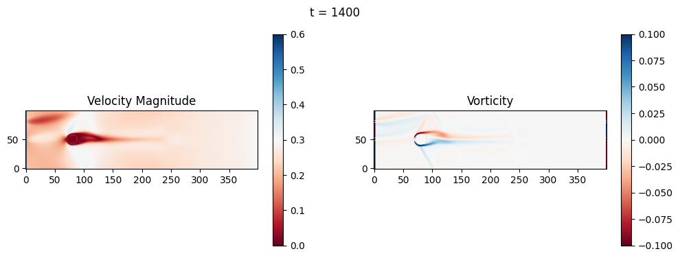
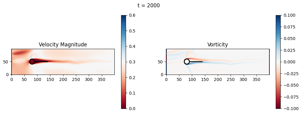
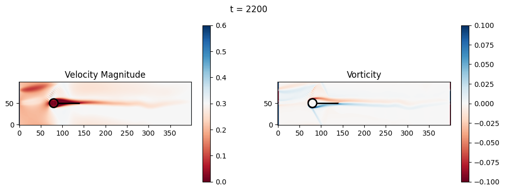
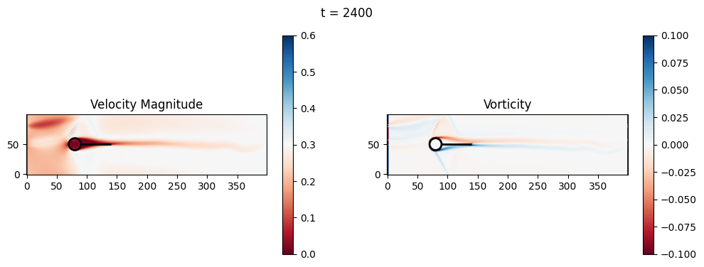
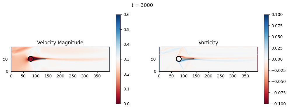
(Optional) Exercise 2: Fluid-solid interaction and basic geometric optimization#
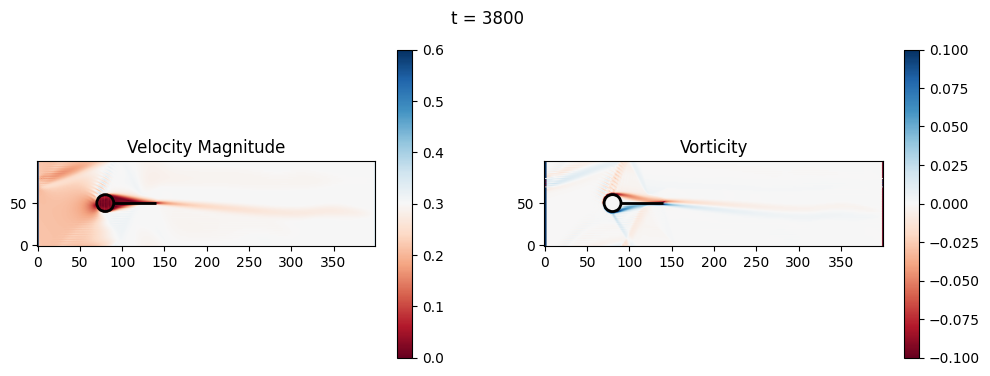
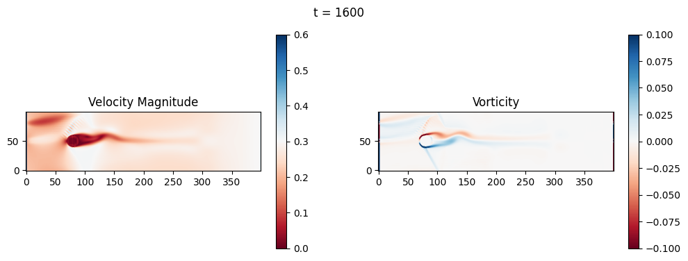
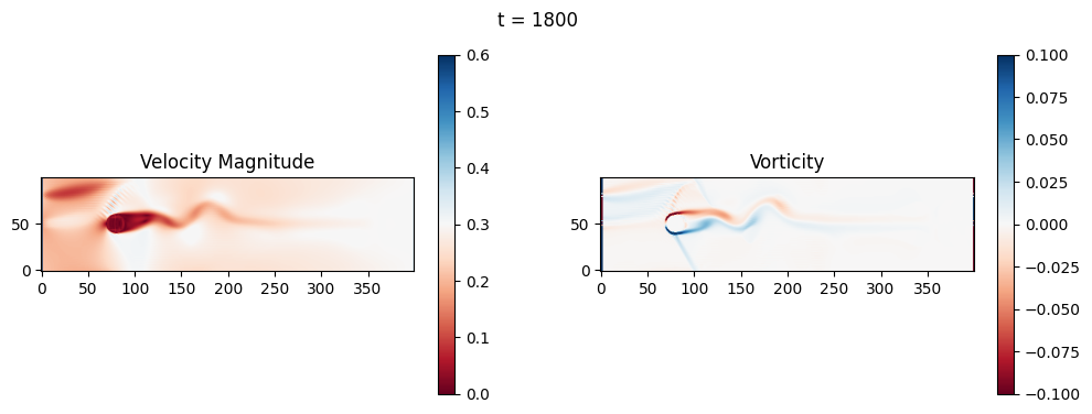
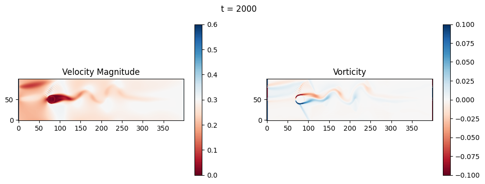
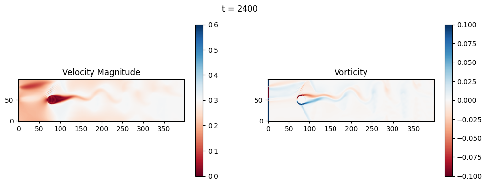
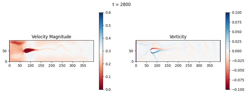
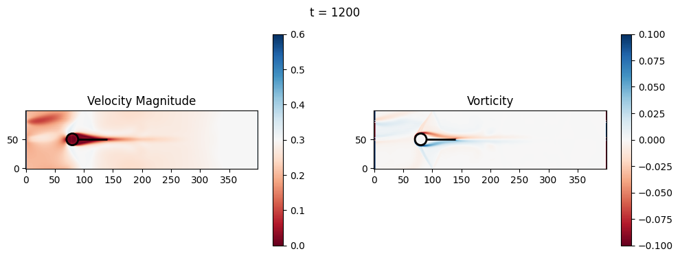
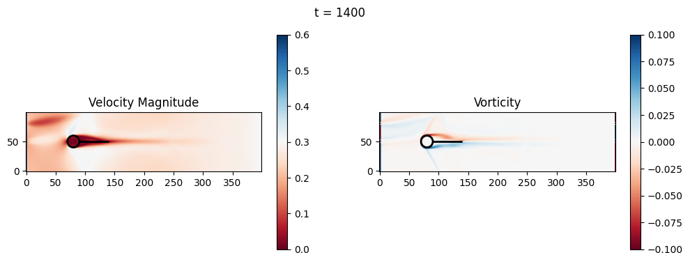
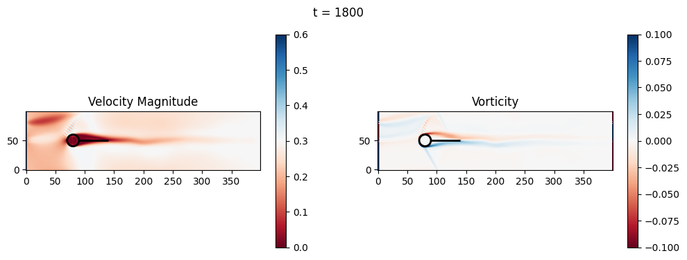
The code below is an LBM (Lattice Boltzmann Method) implementation solving for 2D incompressible fluid low around a cylinder. The second code block also adds a fin which increase
2.1 Compute the Reynold’s number for the case and comment on the regime.
2.2 Adjust the viscosity and cylinder diameter, comment on the results.
2.3 Adjust the length of the fin and comment on the results either qualitatively or quantitatively.
import numpy as np
import matplotlib.pyplot as plt

# Physical parameters
nx, ny = 400, 100  # Grid size
cx, cy, r = nx//5, ny//2, ny//10  # Cylinder position and radius
u_in_max = 0.01  # Even lower for stability
u_in_max = 0.1 # Higher to see vortex shedding
u_in_max = 0.4 # Higher to see vortex shedding
nu = 0.02  # Increased for more viscosity
tau = 3*nu + 0.5  # Relaxation time
#nt = 20000  # Time steps
nt = 4000  # Time steps
plot_every = 200
dx = 1.0  # Lattice spacing

# LBM setup (D2Q9)
w = np.array([4/9, 1/9, 1/9, 1/9, 1/9, 1/36, 1/36, 1/36, 1/36])  # Weights
cx_lbm = np.array([0, 1, 0, -1, 0, 1, -1, -1, 1])  # x velocities
cy_lbm = np.array([0, 0, 1, 0, -1, 1, 1, -1, -1])  # y velocities

# Initialize distributions with uniform flow equilibrium
def equilibrium(rho, ux, uy):
    ux = np.clip(ux, -0.3, 0.3)
    uy = np.clip(uy, -0.3, 0.3)
    if np.isscalar(rho):
        rho = np.array([rho])
        ux = np.array([ux])
        uy = np.array([uy])
    rho = np.asanyarray(rho)
    ux = np.asanyarray(ux)
    uy = np.asanyarray(uy)

    shape = rho.shape
    rho_flat = rho.flatten()
    ux_flat = ux.flatten()
    uy_flat = uy.flatten()
    n = len(rho_flat)

    cu = 3 * (np.tile(cx_lbm[:, None], (1, n)) * np.tile(ux_flat[None, :], (9, 1)) +
              np.tile(cy_lbm[:, None], (1, n)) * np.tile(uy_flat[None, :], (9, 1)))
    uu = 3/2 * (ux_flat**2 + uy_flat**2)
    feq_flat = np.tile(w[:, None], (1, n)) * np.tile(rho_flat[None, :], (9, 1)) * (1 + cu + 0.5*cu**2 - np.tile(uu[None, :], (9, 1)))
    feq_flat = np.nan_to_num(feq_flat)
    feq = feq_flat.reshape(9, *shape)
    return feq

f = equilibrium(np.ones((nx,ny)), np.ones((nx,ny))*0.001, np.zeros((nx,ny)))  # Small initial u for equilibrium

# Cylinder mask
X, Y = np.meshgrid(np.arange(nx), np.arange(ny), indexing='ij')
obstacle = (X - cx)**2 + (Y - cy)**2 <= r**2

def collide(f, rho, ux, uy):
    feq = equilibrium(rho, ux, uy)
    return f - (f - feq) / tau

def stream(f):
    for i in range(1, 9):
        f[i] = np.roll(f[i], shift=(cx_lbm[i], cy_lbm[i]), axis=(0, 1))
    return f

def bounce_back(f, obstacle):
    opp = [0, 3, 4, 1, 2, 7, 8, 5, 6]  # Opposite directions
    f_temp = f.copy()
    for i in range(1, 9):
        f[i, obstacle] = f_temp[opp[i], obstacle]
    return f

def apply_inlet_outlet(f, rho, ux, uy, u_in_current):
    # Inlet (left): Equilibrium BC for smoother
    feq_left = equilibrium(1.0, u_in_current, 0.0)
    f[:, 0, :] = feq_left.squeeze()[:, None]
    # Outlet (right): copy
    f[:, -1, :] = f[:, -2, :]
    return f

def apply_sponge(f, rho, ux, uy):
    # Sponge at outlet (last 20 columns): relax to equilibrium
    sponge_start = nx - 20
    for i in range(sponge_start, nx):
        sigma = (i - sponge_start) / 20.0  # Linear damping
        feq = equilibrium(rho[i, :], ux[i, :], uy[i, :])
        f[:, i, :] = f[:, i, :] * (1 - sigma) + feq * sigma
    return f

# Simulation loop
for t in range(nt):
    # Stream
    f = stream(f)

    # Boundaries
    f = bounce_back(f, obstacle)

    # Macroscopic variables
    rho = np.sum(f, axis=0)
    rho = np.clip(rho, 0.1, 10.0)
    ux = np.sum(f * cx_lbm[:, None, None], axis=0) / rho
    uy = np.sum(f * cy_lbm[:, None, None], axis=0) / rho

    # Ramp inlet velocity (longer ramp)
    u_in_current = u_in_max * min(1.0, t / 1000.0)

    f = apply_inlet_outlet(f, rho, ux, uy, u_in_current)
    f = apply_sponge(f, rho, ux, uy)

    # Collide
    f = collide(f, rho, ux, uy)

    # Wait for the flow to develop before plotting
    if t > 1000:
        if t % plot_every == 0 and t > 0:
            vorticity = (np.roll(uy, -1, axis=0) - np.roll(uy, 1, axis=0)) / (2*dx) - \
                        (np.roll(ux, -1, axis=1) - np.roll(ux, 1, axis=1)) / (2*dx)
            velocity_mag = np.sqrt(ux**2 + uy**2)

            fig, axs = plt.subplots(1, 2, figsize=(12, 4))

            # Velocity magnitude
            im0 = axs[0].imshow(velocity_mag.T, origin='lower', cmap='RdBu', vmin=0, vmax=u_in_max*1.5)
            axs[0].set_title('Velocity Magnitude')
            fig.colorbar(im0, ax=axs[0])

            # Vorticity
            im1 = axs[1].imshow(vorticity.T, origin='lower', cmap='RdBu', vmin=-0.1, vmax=0.1)
            axs[1].set_title('Vorticity')
            fig.colorbar(im1, ax=axs[1])

            fig.suptitle(f't = {t}')
            plt.show()


---------------------------------------------------------------------------
KeyboardInterrupt                         Traceback (most recent call last)
Cell In[21], line 108
    105 f = apply_sponge(f, rho, ux, uy)
    107 # Collide
--> 108 f = collide(f, rho, ux, uy)
    110 # Wait for the flow to develop before plotting
    111 if t > 1000:

Cell In[21], line 55, in collide(f, rho, ux, uy)
     54 def collide(f, rho, ux, uy):
---> 55     feq = equilibrium(rho, ux, uy)
     56     return f - (f - feq) / tau

Cell In[21], line 41, in equilibrium(rho, ux, uy)
     37 uy_flat = uy.flatten()
     38 n = len(rho_flat)
     40 cu = 3 * (np.tile(cx_lbm[:, None], (1, n)) * np.tile(ux_flat[None, :], (9, 1)) +
---> 41           np.tile(cy_lbm[:, None], (1, n)) * np.tile(uy_flat[None, :], (9, 1)))
     42 uu = 3/2 * (ux_flat**2 + uy_flat**2)
     43 feq_flat = np.tile(w[:, None], (1, n)) * np.tile(rho_flat[None, :], (9, 1)) * (1 + cu + 0.5*cu**2 - np.tile(uu[None, :], (9, 1)))

File /opt/hostedtoolcache/Python/3.11.14/x64/lib/python3.11/site-packages/numpy/lib/_shape_base_impl.py:1287, in tile(A, reps)
   1285     for dim_in, nrep in zip(c.shape, tup):
   1286         if nrep != 1:
-> 1287             c = c.reshape(-1, n).repeat(nrep, 0)
   1288         n //= dim_in
   1289 return c.reshape(shape_out)

KeyboardInterrupt:
import numpy as np
import matplotlib.pyplot as plt

# Physical parameters
nx, ny = 400, 100  # Grid size
cx, cy, r = nx//5, ny//2, ny//10  # Cylinder position and radius
u_in_max = 0.01  # Even lower for stability
u_in_max = 0.1 # Higher to see vortex shedding
u_in_max = 0.4 # Higher to see vortex shedding
nu = 0.02  # Increased for more viscosity
tau = 3*nu + 0.5  # Relaxation time
#nt = 20000  # Time steps
nt = 4000  # Time steps
plot_every = 200
dx = 1.0  # Lattice spacing
fin_length = 50  # Trailing fin length (lattice units; adjustable)

# LBM setup (D2Q9)
w = np.array([4/9, 1/9, 1/9, 1/9, 1/9, 1/36, 1/36, 1/36, 1/36])  # Weights
cx_lbm = np.array([0, 1, 0, -1, 0, 1, -1, -1, 1])  # x velocities
cy_lbm = np.array([0, 0, 1, 0, -1, 1, 1, -1, -1])  # y velocities

# Initialize distributions with uniform flow equilibrium
def equilibrium(rho, ux, uy):
    ux = np.clip(ux, -0.3, 0.3)
    uy = np.clip(uy, -0.3, 0.3)
    if np.isscalar(rho):
        rho = np.array([rho])
        ux = np.array([ux])
        uy = np.array([uy])
    rho = np.asanyarray(rho)
    ux = np.asanyarray(ux)
    uy = np.asanyarray(uy)

    shape = rho.shape
    rho_flat = rho.flatten()
    ux_flat = ux.flatten()
    uy_flat = uy.flatten()
    n = len(rho_flat)

    cu = 3 * (np.tile(cx_lbm[:, None], (1, n)) * np.tile(ux_flat[None, :], (9, 1)) +
              np.tile(cy_lbm[:, None], (1, n)) * np.tile(uy_flat[None, :], (9, 1)))
    uu = 3/2 * (ux_flat**2 + uy_flat**2)
    feq_flat = np.tile(w[:, None], (1, n)) * np.tile(rho_flat[None, :], (9, 1)) * (1 + cu + 0.5*cu**2 - np.tile(uu[None, :], (9, 1)))
    feq_flat = np.nan_to_num(feq_flat)
    feq = feq_flat.reshape(9, *shape)
    return feq

f = equilibrium(np.ones((nx,ny)), np.ones((nx,ny))*0.001, np.zeros((nx,ny)))  # Small initial u for equilibrium

# Cylinder mask
X, Y = np.meshgrid(np.arange(nx), np.arange(ny), indexing='ij')
obstacle = (X - cx)**2 + (Y - cy)**2 <= r**2

# Add trailing fin: horizontal line at y=cy, from x = cx + r to cx + r + fin_length
fin_start_x = cx + r
fin_end_x = cx + r + fin_length
fin = (Y == cy) & (X >= fin_start_x) & (X <= fin_end_x)
obstacle = obstacle | fin

def collide(f, rho, ux, uy):
    feq = equilibrium(rho, ux, uy)
    return f - (f - feq) / tau

def stream(f):
    for i in range(1, 9):
        f[i] = np.roll(f[i], shift=(cx_lbm[i], cy_lbm[i]), axis=(0, 1))
    return f

def bounce_back(f, obstacle):
    opp = [0, 3, 4, 1, 2, 7, 8, 5, 6]  # Opposite directions
    f_temp = f.copy()
    for i in range(1, 9):
        f[i, obstacle] = f_temp[opp[i], obstacle]
    return f

def apply_inlet_outlet(f, rho, ux, uy, u_in_current):
    # Inlet (left): Equilibrium BC for smoother
    feq_left = equilibrium(1.0, u_in_current, 0.0)
    f[:, 0, :] = feq_left.squeeze()[:, None]
    # Outlet (right): copy
    f[:, -1, :] = f[:, -2, :]
    return f

def apply_sponge(f, rho, ux, uy):
    # Sponge at outlet (last 20 columns): relax to equilibrium
    sponge_start = nx - 20
    for i in range(sponge_start, nx):
        sigma = (i - sponge_start) / 20.0  # Linear damping
        feq = equilibrium(rho[i, :], ux[i, :], uy[i, :])
        f[:, i, :] = f[:, i, :] * (1 - sigma) + feq * sigma
    return f

# Simulation loop
for t in range(nt):
    # Stream
    f = stream(f)

    # Boundaries
    f = bounce_back(f, obstacle)

    # Macroscopic variables
    rho = np.sum(f, axis=0)
    rho = np.clip(rho, 0.1, 10.0)
    ux = np.sum(f * cx_lbm[:, None, None], axis=0) / rho
    uy = np.sum(f * cy_lbm[:, None, None], axis=0) / rho

    # Ramp inlet velocity (longer ramp)
    u_in_current = u_in_max * min(1.0, t / 1000.0)

    f = apply_inlet_outlet(f, rho, ux, uy, u_in_current)
    f = apply_sponge(f, rho, ux, uy)

    # Collide
    f = collide(f, rho, ux, uy)

    # Wait for the flow to develop before plotting
    if t > 1000:
        if t % plot_every == 0 and t > 0:
            vorticity = (np.roll(uy, -1, axis=0) - np.roll(uy, 1, axis=0)) / (2*dx) - \
                        (np.roll(ux, -1, axis=1) - np.roll(ux, 1, axis=1)) / (2*dx)
            velocity_mag = np.sqrt(ux**2 + uy**2)

            # Downstream region for metrics (x from fin_end_x to nx-50, full y)
            downstream_start = int(fin_end_x) if 'fin_end_x' in locals() else nx//2
            downstream = slice(downstream_start, nx-50)
            vort_mag_down = np.mean(np.abs(vorticity[downstream, :]))
            vel_var_down = np.var(ux[downstream, :] + uy[downstream, :])  # TKE proxy (variance of velocity components)
            print(f"t={t}: Downstream Avg Vorticity Mag = {vort_mag_down:.4f}, TKE Proxy = {vel_var_down:.4f}")

            # Cylinder drag (simple approximation: integrate x-momentum loss around cylinder)
            cyl_slice = slice(cx - r - 5, cx + r + 5)
            drag_approx = np.sum(rho[cyl_slice, :] * ux[cyl_slice, :] * dx)  # Proxy for drag (momentum flux)
            print(f"t={t}: Cylinder Drag Proxy = {drag_approx:.4f}")

            fig, axs = plt.subplots(1, 2, figsize=(12, 4))

            # Velocity magnitude
            im0 = axs[0].imshow(velocity_mag.T, origin='lower', cmap='RdBu', vmin=0, vmax=u_in_max*1.5)
            axs[0].set_title('Velocity Magnitude')
            fig.colorbar(im0, ax=axs[0])

            # Add black lines for cylinder and fin
            circle = plt.Circle((cx, cy), r, color='black', fill=False, linewidth=2)
            axs[0].add_patch(circle)
            axs[0].hlines(cy, fin_start_x, fin_end_x, colors='black', linewidth=2)

            # Vorticity
            im1 = axs[1].imshow(vorticity.T, origin='lower', cmap='RdBu', vmin=-0.1, vmax=0.1)
            axs[1].set_title('Vorticity')
            fig.colorbar(im1, ax=axs[1])

            # Add black lines for cylinder and fin
            circle = plt.Circle((cx, cy), r, color='black', fill=False, linewidth=2)
            axs[1].add_patch(circle)
            axs[1].hlines(cy, fin_start_x, fin_end_x, colors='black', linewidth=2)

            fig.suptitle(f't = {t}')
            plt.show()
t=1200: Downstream Avg Vorticity Mag = 0.0012, TKE Proxy = 0.0004
t=1200: Cylinder Drag Proxy = 388.5402
t=1400: Downstream Avg Vorticity Mag = 0.0016, TKE Proxy = 0.0005
t=1400: Cylinder Drag Proxy = 383.9169
t=1600: Downstream Avg Vorticity Mag = 0.0021, TKE Proxy = 0.0009
t=1600: Cylinder Drag Proxy = 376.9995

t=1800: Downstream Avg Vorticity Mag = 0.0024, TKE Proxy = 0.0011
t=1800: Cylinder Drag Proxy = 376.9451
t=2000: Downstream Avg Vorticity Mag = 0.0024, TKE Proxy = 0.0010
t=2000: Cylinder Drag Proxy = 377.3504
t=2200: Downstream Avg Vorticity Mag = 0.0024, TKE Proxy = 0.0008
t=2200: Cylinder Drag Proxy = 378.1023
t=2400: Downstream Avg Vorticity Mag = 0.0024, TKE Proxy = 0.0006
t=2400: Cylinder Drag Proxy = 378.1402
t=2600: Downstream Avg Vorticity Mag = 0.0023, TKE Proxy = 0.0006
t=2600: Cylinder Drag Proxy = 379.1670

t=2800: Downstream Avg Vorticity Mag = 0.0022, TKE Proxy = 0.0005
t=2800: Cylinder Drag Proxy = 383.2964

t=3000: Downstream Avg Vorticity Mag = 0.0019, TKE Proxy = 0.0004
t=3000: Cylinder Drag Proxy = 388.4117
t=3200: Downstream Avg Vorticity Mag = 0.0016, TKE Proxy = 0.0003
t=3200: Cylinder Drag Proxy = 386.6070

t=3400: Downstream Avg Vorticity Mag = 0.0015, TKE Proxy = 0.0003
t=3400: Cylinder Drag Proxy = 386.6438

t=3600: Downstream Avg Vorticity Mag = 0.0015, TKE Proxy = 0.0003
t=3600: Cylinder Drag Proxy = 386.1305

t=3800: Downstream Avg Vorticity Mag = 0.0014, TKE Proxy = 0.0002
t=3800: Cylinder Drag Proxy = 386.1483